


The HSTACK function in Google Sheets is for appending ranges horizontally. Even though we can use Curly Braces for this purpose, it can’t substitute the HSTACK function.
Do you know the reason?
The Curly Braces requires all the ranges to append must contain an equal number of rows.
But in the HSTACK function, we can use arrays of any size. It does not necessarily match the columns and rows in the appending ranges.
I find VSTACK (vertical stacking) more practical when compared to HSTACK (horizontal stacking), its sibling.
Syntax of the HSTACK Function
Syntax: HSTACK(range1; [range2, …])
range1: The first array or range to append.
range2, … : Additional arrays or ranges (optional) to add to the previous range.
Example
I’ve three tables and want to append them horizontally into a single array.
The table ranges are A3:D4, A6:C8, and A9:D10.
The HSTACK formula in cell A13 returns the single appended array in A13:K15.
=hstack(A3:D4,A6:C8,A10:D11)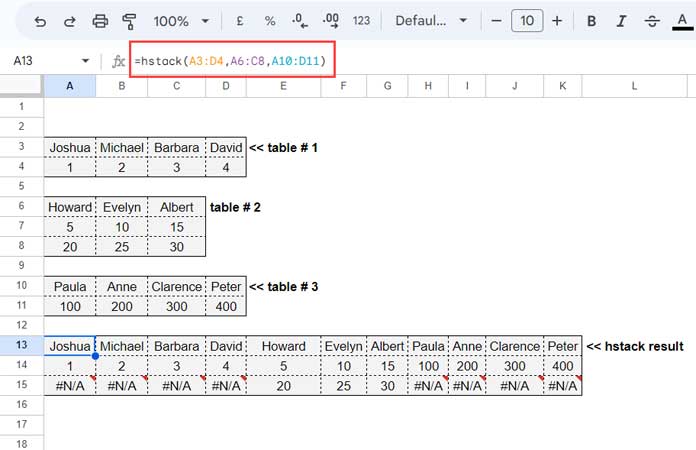
What’s the reason for a few #N/A values in the result?
As you can see, the number of rows and columns is different in each table.
But the HSTACK function has no issue in appending them horizontally.
The HSTACK formula output will have the number of rows matching the max number of rows in the appended ranges.
In the process, it adds #N/A values in some cells.
To remove them, wrap the formula with an IFERROR.
=iferror(hstack(A3:D4,A6:C8,A10:D11))HSTACK with SUMIF Function in Google Sheets (Real-Life Use)
We have learned how the HSTACK function works in Google Sheets.
In the following real-life use example, I will use it with SUMIF to generate a summary table.
Assume we have a product list in column A and their quantities in column B.
How do we make a summary out of it?
Of course, the following QUERY formula will do that.
=query(A:B,"Select A, sum(B) where A is not null group by A",1)Alternatively, we can use UNIQUE and SUMIF as follows.
=hstack(tocol(unique(A2:A),3),index(sumif(A2:A,tocol(unique(A2:A),3),B2:B)))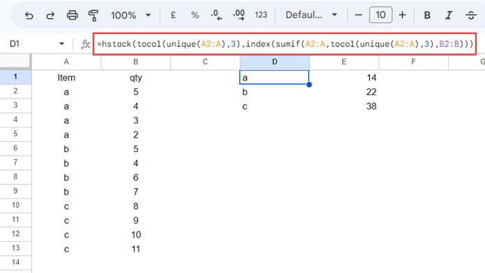
We can split and learn this last formula.
range1: tocol(unique(A2:A),3)
range2: index(sumif(A2:A,tocol(unique(A2:A),3),B2:B))
The range1 in the above HSTACK formula returns the unique items without blanks.
The range2 returns the summary of the unique items.
I hope the above examples help you learn the use of the HSTACK function in Google Sheets.