There are three main wildcard characters in Google Sheets that you can use with certain functions: ‘~’ (tilde), ‘*’ (asterisk), and ‘?’ (question mark).

Please do not confuse the term ‘wildcard’ with the term ‘wild card.’ The former applies to computer technology (wildcard character), whereas the latter has a different meaning in sports events (for example, wild card entry).

This tutorial focuses on the use of the tilde, asterisk, and question mark symbols (special characters) in formulas within Google Sheets.

These individual wildcard characters (the three symbols mentioned above) can represent or replace single or multiple other characters in formulas. Here are their purposes.

• Asterisk (*): Matches a variable number of characters.
• Question Mark (?): Matches a single character.
• Tilde (~): Serves as an escape character for another wildcard when positioned in front of it, transforming it into a literal character instead.

Let me take you through a few examples to help you understand the proper use of wildcards in Google Sheets.

Wildcards in Google Sheets

We can learn how to use the three wildcard characters mentioned above in Google Sheets formulas, rather than in the search or find and replace command

I am using the basic forms of two Google Sheets functions in the examples to help you understand the use of wildcards in Google Sheets.

Additionally, there are separate tutorials for the advanced use of some of the symbols mentioned above, which you can find in the last part of this tutorial.

In the examples below, I will be using the symbols with the SUMIF and SUMIFS functions. You can follow the same procedures to apply wildcards in other supported functions. Hence, I will not repeat the steps for every function here.

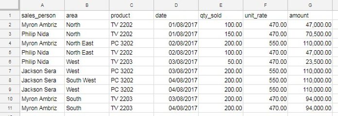
We will use the following sample data (please refer to the screenshot below) for the examples. It contains the names of salespersons, the area they operate in, the products they sell, the date of sale, quantity sold, unit rate, and amount, arranged in columns A to G. You can click on the button immediately after the image to obtain a copy of my sample sheet.

Sample Sheet

SUMIF Partial Match

Are you looking for a criterion-based sum? Then, this is the function you are searching for! No doubt, the QUERY function is available, and even SUM + FILTER will also work. However, SUMIF is simple to understand and use.

Syntax: SUMIF(range, criterion, [sum_range])

Use of Wildcard Character Question Mark (?) with SUMIF

The question mark wildcard character in the SUMIF formula in Google Sheets can represent or take the place of any single character in the criterion part.

We can use the symbol twice (or more) in case we want to represent two unknown characters. You can find both examples below.

=SUMIF(C2:C11, "TV 2202", G2:G11)

The above SUMIF formula is used to sum the ‘amount’ if the ‘product’ is “TV 2202”. No wildcard character is used in this Google Sheets formula.

Here is a slightly different formula that contains the question mark symbol.

=SUMIF(C2:C11, "TV 220?", G2:G11)

This formula will sum the ‘amount’ if the ‘product’ matches “TV 2202” or “TV 2203” based on our sample data.

The last character is not important here, but there should be one character followed by “TC 220”. That’s important.

With one more example, we can conclude this part. Here is a formula having multiple wildcards in Google Sheets.

=SUMIF(C2:C11, "TV 22??", G2:G11)

Here, the text can be “TV 2201” or “TV 2202”. What’s important here is that there should be two characters, no matter which two characters, followed by “TV 22”.

Use of Wildcard Character Asterisk (*) with SUMIF

The asterisk symbol can represent or take the place of any number of characters in the criterion part in SUMIF.

Here are two examples:

=SUMIF(C2:C11, "TV*", G2:G11)

The above formula is used to sum the ‘amount’ if the ‘product’ is “TV2202”, “TV 2203456”, or any word starting with “TV.”

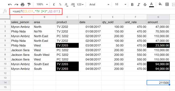
In the formula below, it can be any text but should start with “TV 2” and end with “3”. That means “TV 244444443”, “TV 2111113”, etc.

=SUMIF(C2:C11, "TV 2*3", G2:G11)

Use of Wildcard Character Tilde (~) with SUMIF

The use of this wildcard character in Google Sheets (inside the SUMIF function) is entirely different compared to the above two and can be a bit confusing.

Sometimes, when your text includes “?” or “*” as regular characters, you can prefix them with a tilde (~) to make them literal characters instead of wildcards.

In the following example, the ‘?’ is considered a literal character, not a wildcard character.

=SUMIF(B2:B11, "No~?th", G2:G11)

SUMIFS Partial Match

Similar to SUMIF, for summing based on multiple criteria, we can rely on SUMIFS, SUM + FILTER, or QUERY.

Syntax: SUMIFS(sum_range, criteria_range1, criterion1, [criteria_range2, …], [criterion2, …])

Here are some examples of partial matching in SUMIFS in Google Sheets.

Use of Wildcard Character Question Mark (?) with SUMIFS

Similar to SUMIF, this wildcard character can represent or take the place of any single character.

=SUMIFS(G2:G11, B2:B11, "North", C2:C11, "TV 2202")

In the above SUMIFS formula, no wildcard characters are used. The formula is to sum the ‘amount’ if the ‘area’ is “North” and the ‘product’ is “TV 2202”.

What about this one?

=SUMIFS(G2:G11, B2:B11, "North", C2:C11, "TV 22??")

Here I have used the question mark wildcards in Google Sheets with one of the SUMIFS conditions (criterion).

This formula is to sum the ‘amount’ if the ‘area’ is “North” and the ‘product’ is “TV 2202” or any text, but the starting characters should be “TV 22” followed by two more characters.

Use of Wildcard Character Asterisk (*) with SUMIFS

This wildcard character in SUMIFS can represent or take the place of any number of characters.

Straight to one example.

=SUMIFS(G2:G11, B2:B11, "*East", C2:C11, "TV*")

This SUMIFS formula sums the ‘amount’ if the ‘area’ is either “North East” or “South East” (as per our sample data) and the ‘product’ is any text starting with “TV”.

Use of Wildcard Character Tilde (~) with SUMIFS

The following formula sums the ‘amount’ if the ‘area’ is “No?th” and the ‘product’ is any item starting with “TV”:

=SUMIFS(G2:G11, B2:B11, "No~?th", C2:C11, "TV*")

If you haven’t specified the tilde, the formula matches “North” along with “No?th” and returns a different output.

Wildcards in Other Functions in Google Sheets

The examples above demonstrate the use of wildcards in SUMIF and SUMIFS in Google Sheets.

What about other Google Sheets functions?

You may be able to use the above three special characters for partial matches in most formulas that use criteria. However, there are exceptions and additional steps.

In XLOOKUP and XMATCH, two modern lookup functions, you can use wildcard characters, but only in ‘search mode 2.’

The FILTER function uses criteria for filtering tables, but it doesn’t support wildcards. However, you can achieve that with a workaround using the SEARCH function. You may also be able to use REGEXMATCH instead of SEARCH.

Additionally, the IF logical function doesn’t support the above special characters. In the “Resource” section below, see how to address this issue.

Resources

The following tutorials discuss partial matching in Google Sheets. Some formulas in them utilize wildcard characters, while others employ the SEARCH or REGEXMATCH functions. I hope you find them useful.

1. Partial Match in IF Function in Google Sheets As Wildcard Alternative
2. Partial Match in Vlookup in Google Sheets [Text, Numeric, and Date]
3. CONTAINS Substring Match in Google Sheets Query for Partial Match
4. Lookup Last Partial Occurrence in a List in Google Sheets
5. Wildcards in Vlookup Search Range in Google Sheets
6. LIKE String Operator in Google Sheets Query and Wildcard Use
7. Filter Out Matching Keywords in Google Sheets – Partial or Full Match
8. Regexmatch in Filter Criteria in Google Sheets [Examples]
9. REGEXMATCH in SUMIFS and Multiple Criteria Columns in Google Sheets
10. How to Use Wildcards in Sumproduct in Google Sheets