Using the ACCRINTM function in Google Sheets, we can calculate the accrued interest or interest accumulated for a security that pays interest only at maturity.
The letter M at the end of this financial function denotes maturity. Needless to say, ACCR is taken from accrued, and INT is taken from interest.
As a side note, it is a good idea to name functions like this so that we can easily remember them. You can follow this when naming Named functions in Google Sheets.
If the interest (coupon payment) is paid periodically, there is a different function called ACCRINT, which I explained in another tutorial.
ACCRINTM Function in Google Sheets: Syntax and Arguments
Syntax of the ACCRINTM Function in Google Sheets:
ACCRINTM(issue, maturity, rate, [redemption], [day_count_convention])Arguments:
issue: The issue date of the security.maturity: The date the security matures.rate: The annualized rate of interest.redemption: The par value of the security. If you omit par, the function will use $1,000. It’s an optional argument.day_count_convention: An indicator of what day count method to use. By default, it is 0 (zero), which is the US (NASD) 30/360 convention. It’s an optional argument.
Day_Conunt_Convention Table:
| Indicator | Description |
| 0 | US (NASD) 30 days months / 360 days years |
| 1 | Actual / Actual |
| 2 | Actual / 360 days years |
| 3 | Actual / 365 days years |
| 4 | European 30 days months / 360 days years |
Note: The ACCRINT function (not ACCRINTM) uses the settlement date and first coupon payment date instead of the maturity date. We should also specify the frequency of the coupon payments, as the function is for accrued interest of securities with periodic payments.
How to Use the ACCRINTM Function in Google Sheets
Example of using the ACCRINTM function in Google Sheets:
Assume you borrowed $15,000 from a bank to finance one of your new projects. The loan has a 7-year term from January 1, 2015, to January 1, 2022, and an interest rate of 12%.
We can use the ACCRINTM function to calculate the interest that accrues on the loan balance, which is paid back to the bank when the loan matures:
=ACCRINTM(DATE(2015, 1, 1), DATE(2022, 1, 1), 12%, 15000, 3) // In this case, the accrued interest would be: $12,609.86Where:
DATE(2015, 1, 1)is theissuedate in the syntaxDATE(year, month, day).DATE(2022, 1, 1)is thematuritydate in the syntaxDATE(year, month, day).12%is the annual interestrateof the loan.15000is theredemption(here, loan) amount.3is theday_count_convention.
Note: The “issue” and “maturity” arguments should be entered using the DATE function as above. This is to avoid date formatting issues such as DD/MM/YYYY and MM/DD/YYYY.
It is better to enter the input values within the sheet and refer to them in the ACCRINTM formula, as follows:
=ACCRINTM(B1,B2,B3,B4,B5)Where:
B1is the cell reference of the cell containing theissuedate.B2is the cell reference of the cell containing thematuritydate.B3is the cell reference of the cell containing the interestrate.B4is the cell reference of the cell containing the loan amount (redemption).B5is the cell reference of the cell containing theday_count_convention.
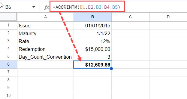
This makes the formula more readable and easier to maintain.
Accrued Interest Formula Explained: How to Calculate Accrued Interest Step-by-Step
We have seen how to use the ACCRINTM function to calculate accrued interest in Google Sheets. To do this, we simply need to input the required parameters. Here is how to calculate accrued interest without using the function using those parameters:
Accrued interest = Principal amount * Interest rate * (Number of days from the issue date to the maturity date / n)For example, if we have a principal amount of $15,000 and an interest rate of 12%, then the accrued interest would be calculated as follows:
=15000*12%*(DAYS(DATE(2022,1,1),DATE(2015,1,1))/365) // The result is 12609.86Where:
- The
15000is the amount of the loan. 12%is the annual interest rate on the loan.- The
DAYS(DATE(2022,1,1),DATE(2015,1,1))is the number of days between the date the loan was issued [DATE(2015,1,1)] and the date the loan is due to be repaid [DATE(2022,1,1)].- The syntax of the DAYS function is
DAYS(end_date, start_date), which returns the number of days between two dates.
- The syntax of the DAYS function is
365is the year part of the day count convention.
In this example, we are using the “Actual / 365 days years” day count convention, which assumes that there are 365 days in a year. Therefore, n is 365.
Conclusion
Before wrapping up, let me point out two common errors that you might see when using the ACCRINTM financial function in Google Sheets:
1. VALUE! error in ACCRINTM:
- Cause: Invalid issue date or maturity date.
- Solution: Use the DATE function if the issue or maturity date is entered directly in the formula. If you are using cell references, make sure that the dates are in the correct format (
DD/MM/YYYYorMM/DD/YYYY).
2. NUM! error in ACCRINTM:
Causes:
- The rate is less than or equal to 0.
- The par value is less than or equal to 0.
- The day count indicator is out of range (the range is 0 to 4).
- The issue date is greater than or equal to the maturity date.
Solution: Make sure that all of the arguments to the ACCRINTM function are valid.


