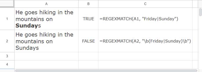
We can use the REGEXMATCH function for complex substring matching in Google Sheets, as it utilizes regular expressions for matching.
REGEXMATCH returns Boolean values (TRUE or FALSE), which can be used as conditions in other functions. Understanding this function is important as it can be combined or nested with functions like FILTER, COUNTIFS, SUMIFS, etc.
Two other functions use regular expressions: REGEXEXTRACT and REGEXREPLACE. Their names suggest their purposes.
Syntax:
REGEXMATCH(text, regular_expression)text– The text to be tested against the regular expression pattern.regular_expression– The regular expression pattern used to test the text.
Formula Examples: REGEXMATCH Most Common Use Cases
Here are some common use cases. Once you’ve learned them, you can advance further by referring to the RE2 regular expression syntax reference on GitHub. Google Sheets supports RE2 syntax, excluding Unicode character class matching.
Also, note that all examples are case-sensitive. After the examples, I’ll share how to make them case-insensitive.
Example 1: Match Substrings within a String
Enter the following string in cell A1:
He visited the site last Friday and Saturday
How do you find out whether this string contains the substring “Friday” or not?
You can use the following REGEXMATCH formula in cell B1:
=REGEXMATCH(A1, "Friday")This will return TRUE since the cell contains “Friday”.
When you want to match multiple substrings within a string, you can separate each substring with a pipe in the regular expression:
=REGEXMATCH(A1, "Friday|Sunday")If either substring is present, the formula will return TRUE.
If you replace the string in cell A1 with the following one, the formula will still return TRUE:
He goes hiking in the mountains on Sundays
Because the substring “Sunday” partially matches.
What if you want to exactly match the substring within a string using the REGEXMATCH function in Google Sheets?
Formula:
=REGEXMATCH(A1, "\b(Friday|Sunday)\b") // returns FALSEWhere \b asserts the position at a word boundary.

Example 2: Match Content within Two Specific Characters Such as Brackets
This is another common use case of the REGEXMATCH function in Google Sheets.
For example, you might want to match specific text within an array such as {500, 400, 4001, 250, 300}. How do you do that?
=REGEXMATCH(A1, "\{.*400\,.*\}")It will match the substring 400, and return TRUE since it is present in the text.
In this formula, you can replace {} with (), [], or <> to match a specific substring within them.
Explanation:
\{matches the character{..*matches any character (.) any number of times (*).400\,matches the characters400,.\}matches the character}.
Example 3: REGEXMATCH for Exact Match of Multiple Strings
This is another common use case of the REGEXMATCH function, especially when used with functions such as FILTER, SUMIFS, COUNTIFS, etc.
If cell A1 contains the string “pineapple,” the following formula will return TRUE as it partially matches “apple” in “pineapple”:
=REGEXMATCH(A1, "apple") // returns TRUEHow do you match them exactly?
=REGEXMATCH(A1, "^apple$") // returns FALSEWhere ^ asserts the position at the start of a line and $ at the end of the line.
When you want to match multiple strings exactly, specify them separated by a pipe as follows:
=REGEXMATCH(A1, "^apple$|^orange$|^mango$")When you want to REGEXMATCH values in a range, use the ARRAYFORMULA function. In the following example, the formula uses the above regular expression to test the range A1:A5:
=ArrayFormula(REGEXMATCH(A1:A5, "^apple$|^orange$|^mango$"))
Other Common Patterns in Use
Here are some other common regular expression patterns that you may encounter in Google Sheets formulas:
(\d): matches digits[0-9]: matches digits[a-z]: matches the character range a-z, inclusive[A-Z]: matches the character range A-Z, inclusive
For case-insensitive matches, specify (?i) in front of the patterns. For example, use the following formula to match multiple values in a range case-insensitively:
=ArrayFormula(REGEXMATCH(A1:A5, "(?i)^apple$|^orange$|^mango$"))As a side note, I am skipping email address validation since there is a dedicated function called ISEMAIL in Google Sheets.
An Example of the REGEXMATCH Function in Real-Life Use in Google Sheets
When you have a list of household items in column A and their quantities in column B, you can use the following SUMIF formula to find the total quantities of “Sofa” and “Dining Table”:
=ArrayFormula(SUMIF(REGEXMATCH(A2:A, "Sofa|Dining Table"), TRUE, B2:B))It follows the syntax: SUMIF(range, criterion, [sum_range])
Where:
range:ArrayFormula(REGEXMATCH(A2:A, "Sofa|Dining Table"))criterion:TRUEsum_range:B2:B
Resources
- REGEXMATCH in Filter Criteria in Google Sheets [Examples]
- REGEXMATCH in SUMIFS and Multiple Criteria Columns in Google Sheets
- REGEXMATCH Dates in Google Sheets – Single/Multiple Match
- How to Use REGEXMATCH in AVERAGEIF in Google Sheets
- Case-Insensitive REGEXMATCH in Google Sheets (Part or Whole)
- NOT in REGEXMATCH and Alternatives in Google Sheets
- Matches Regular Expression Match in Google Sheets Query


Good day to you.
I am using the following formula:
=ARRAYFORMULA(IFERROR(REGEXMATCH(FLATTEN(AT7:INDIRECT(AT1&AT2)),JOIN("|",AV7:INDIRECT(AV1&AV2))),""))The challenge:
“T” should generate True
“TB” should generate False
However, “TB” is currently generating True.
Is it possible to modify the formula to ensure an exact match?
Thanks.
I recommend using TEXTJOIN instead of JOIN to avoid errors associated with empty cells.
Here’s my suggested formula, where I replaced AV with A and AT with B:
=ARRAYFORMULA(IFERROR(REGEXMATCH(FLATTEN(A7:INDIRECT(A1&A2)), "^"&TEXTJOIN("$|^", TRUE, B7:INDIRECT(B1&B2))&"$"),""))Thanks. That works.
I have tried the examples here in relation to a workbook I am using and they all return parse errors.
Any suggestions as to where to check appreciated.
Hi, CJ,
It may due to LOCALE settings. Replace the comma in your formula with a semicolon.
I want to match inside query the expression:
6.1)How can I do that, I’ve tried:
matches '6.1)'– not workingmatches '\6.1\)'– not workingmatches '\6.1)\)'– not workingPlease help
Hi, Jofre Navarrete,
I assume you were talking about the Matches Regular Expression Match in Google Sheets Query.
In that case the formula would be as below.
=query(C1:D,"Select D where D matches '6.1\)'")You only need to escape the closing bracket.
Thank You Prashanth