When you want to identify top performers in a dataset in Google Sheets, the RANK function is what you need to use.

There are two other similar functions: RANK.AVG and RANK.EQ. Let’s quickly overview how they differ before diving into the syntax and examples of the RANK function.

• RANK: Returns the rank of a specified value in an array or range.
• RANK.AVG: Similar to RANK but returns the average rank of the value if it appears multiple times.
• RANK.EQ: Replaces the RANK function. Both functions can be used interchangeably.

To understand these functions better, consider the rank of the value 100 in a dataset. As it tops the list, it is ranked #1.

If 100 appears four times, the RANK and RANK.EQ functions will return 1, whereas RANK.AVG will return 2.5.

RANK Function: Syntax and Arguments

RANK Function Syntax in Google Sheets:

RANK(value, data, [is_ascending])

Arguments:

• value: The value whose rank you want to find. If the specified value is not present, the formula will return #N/A, which you can handle using an IFNA wrapper.
• data: The array or range to consider. It can be either one-dimensional or two-dimensional, but it should be of equal size.
• is_ascending: An optional but important argument. You can specify either 0 or 1. If omitted, the value defaults to 0.
  • If 0, rank #1 will go to the greatest value.
  • If 1, rank #1 will go to the least value.

Understanding Ranking from Top to Bottom and Bottom to Top

Take a look at the following three formulas which return the rank of 10 in the array {1, 2, 3, 4, 5, 6, 7, 8, 9, 10}:

=RANK(10, {1, 2, 3, 4, 5, 6, 7, 8, 9, 10})
=RANK(10, {1, 2, 3, 4, 5, 6, 7, 8, 9, 10}, 0)
=RANK(10, {1, 2, 3, 4, 5, 6, 7, 8, 9, 10}, 1)

The first two formulas will return 1, which is the rank of 10 in the array because the greatest value gets rank #1.

The last formula will return the rank 10 because the least value gets rank #1.

Ranking Students by Total Marks: Applying RANK with ARRAYFORMULA

In the following example, I have student names in A2:A5 and their total marks in F2:F5. To find their rank, we can use the following RANK array formula in cell G2.

=ArrayFormula(RANK(F2:F5, F2:F5, 0))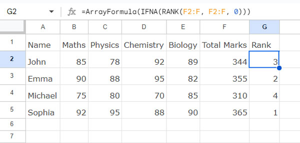

If you specify open ranges, wrap the formula with IFNA since the ‘value’ shouldn’t be empty.

=ArrayFormula(IFNA(RANK(F2:F, F2:F, 0)))

Open ranges result in empty value cells, causing the RANK function to return #N/A. Using IFNA helps remove such errors.

RANK Function in Visible Rows in Google Sheets

The RANK function can’t return the rank of values in visible rows only. However, in Google Sheets, you can follow the approach below to exclude hidden rows when returning the rank of values in a dataset.

For example, let’s consider the marks of students provided above. You can use the following formula in cell G2 to return the rank of visible values in the dataset:

=ArrayFormula(LET(values, F2:F5, visible_rows, MAP(values, LAMBDA(r, SUBTOTAL(103, r))), visible_values, IF(visible_rows, values, ), RANK(visible_values, visible_values)))

In this formula, F2:F5 is the reference corresponding to the total marks.

When you hide or filter out any rows, the formula will exclude values in corresponding cells in F2:F5 from the rank calculation.

Formula Breakdown

visible_rows: This part identifies visible rows by returning 1 for visible rows and 0 for hidden rows.

• LAMBDA(r, SUBTOTAL(103, r)): A custom LAMBDA function that returns the count of values in the current row in the data.
• MAP(values, LAMBDA(r, SUBTOTAL(103, r))): The MAP function iterates the custom function for each value in the array, where the array is F2:F5, named ‘values’ using LET. The output will be 1 for visible rows and 0 for hidden rows, corresponding to F2:F5.

visible_values: This part empties hidden cells virtually.

• IF(visible_rows, values, ): If a row is visible (contains a count of 1, as hidden rows have a count of 0), the formula returns the values (marks); otherwise, it returns blank.

RANK(visible_values, visible_values): The RANK function returns the ranks of all values but ignores values in hidden rows, as they are converted to empty in the previous step.

Resources

• How to Find the Rank of a Non-Existing Number in an Existing Data Range
• Flexible Array Formula to Rank Without Duplicates in Google Sheets
• How to Rank Group Wise in Google Sheets in Sorted or Unsorted Group
• Top 10 Ranking without Duplicate Names in Google Sheets
• Compare and Highlight Up and Down in Ranking in Google Sheets
• Find the Rank of an Item in Each Column in Google Sheets
• Highlight the Top 10 Ranks in Single or Each Column in Google Sheets
• How to Rank without Ties in Google Sheets
• How to Rank Data by Alphabetical Order in Google Sheets
• How to Rank Text Uniquely in Google Sheets