Let’s see How to Highlight Only Texts in Google Sheets. Some of you may ask why should one highlight only texts or strings? There is a specific reason! Just read on to understand that.
I am going to post a few Google Sheets tutorials related to conditional formatting. Conditional formatting can play a vital role in data cleaning and with this tutorial, I’m trying to give you some idea in that direction.
In this conditional formatting tutorial, you can learn how to highlight only texts in Google Sheets either in Row-wise, Column-wise or in an entire sheet.
For this purpose I’m making use of the Regexmatch formula. You just need to apply the custom formula which I’m going to provide you here and that part I’ll explain below.
How to Highlight Only Texts in Google Sheets
The custom formula to highlight only texts in a column, row or an entire sheet is as below.
=ArrayFormula(REGEXMATCH(A1:A,"[a-zA-Z]"))
Here you just need to replace the range A1: A as per your requirement. In this Google Sheets tutorial, I’ve selected Column A and that’s why the range is so in the formula.
Now let us see how to apply this custom formula in Conditional Formatting.
Steps to Highlight Only Texts in a Column in Google Doc Spreadsheets:
1. Select the range, row or column first. In my example, I’m applying this conditional formatting rule to Column A.
2. Then go to the menu Format > Conditional formatting.
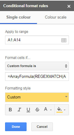
3. You can see the conditional formatting rules panel. Make sure that “Apply to range” is the correct range where you want the conditional formatting to apply.
4. From the drop-down under “Format cells if…” select “Custom formula is…” and paste our above Regex formula. Change the range in the formula if necessary.
5. Now under “Formatting style” you can see different formatting options. You can change the font color, highlight the cell by filling color etc. Once you complete the above steps, click “Done”

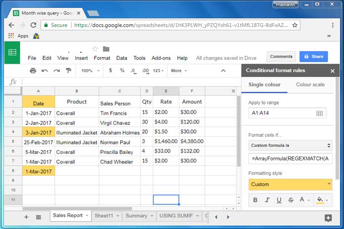
You can see the final result as below. Bizarre, right?
You can see that I’ve applied the above conditional formatting rule in a column that containing the date.
Again when you cross-check the column, you can further see that the conditional formatting rule highlighted certain cells containing dates. But our rule is to highlight Only Texts in a Column, right? Then why this has happened?
Below is the answer.

How to Find Cells Containing Invalid Date Format in Google Sheets
Actually, my tutorial is discussing how to highlight only texts in a Column or Row in Google Sheets. I have done it correctly. But my purpose of the highlighting was different! I want to find cells containing invalid dates in a column.
In Column A, Cell A4 and A8 are containing texts, not dates. I mean they are dates formatted as text. So it would only behave like a text string.
That means, in a date wise calculation, that text values may cause an invalid result. So with this conditional formatting rule, I could able to find the invalid data entries, i.e. dates entered as text and I can correct that easily now.


