To filter integers (whole numbers) in a list, you can use the FILTER function in Google Sheets. The filtered results will be displayed in a new range. You can also apply the filter to the same list by using a custom formula in the Data menu > Create a filter.
In addition to this, in this tutorial, you will also learn how to:
- Highlight whole numbers: You can use the Conditional Formatting feature to highlight all the cells that contain integers.
- Mark the rows containing whole numbers in a new column: You can use an IF logical test to create a new column that contains a value of TRUE if the cell in the original column contains an integer and FALSE if the cell does not contain an integer.
How to Filter Integers in Google Sheets with the FILTER Function
The syntax of the FILTER function is:
FILTER(range, condition1, [condition2, …])Assuming the list is in the range B1:B and B1 contains the field label, you can use the following FILTER formula to filter integers in this array:
=FILTER(B2:B, B2:B = INT(B2:B))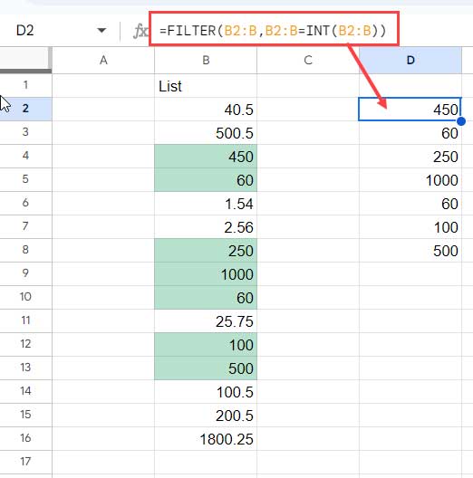
Where:
B2:Bis the range of cells to be filtered.B2:B = INT(B2:B)is the condition that the cells in the range must meet. This condition checks if the value in each cell is an integer.
The role of the INT function here is to convert the numbers in the array to integers. The formula compares the converted values to the original values and returns the matching values.
This is an array formula that returns multiple values based on the number of whole numbers in the list.
Since the range is vertical, the formula returns multiple rows. Ensure that there are sufficient blank cells below the cell where the formula is applied. Otherwise, it will return a #REF! error, which cannot be resolved by wrapping the formula with an IFERROR function.
How to Filter Integers in Google Sheets with the Filter Menu
As you can see in our earlier example, the formula returns the output in a new range. However, if you want to filter the source list, use the Data > Create a filter command.
First, you need to apply the filter to the list. To do this, select the range B1:B, then go to Data > Create a filter. Alternatively, you can right-click on cell B1 and choose Create a filter from the shortcut menu.
Then, follow these five steps to apply the custom formula to filter the integers in the list:
- Click on the filter dropdown menu icon (filter icon) in cell
B1. - Select Filter by condition.
- Choose Custom formula is.
- Enter
=B2=INT(B2)in the provided field. - Click OK.
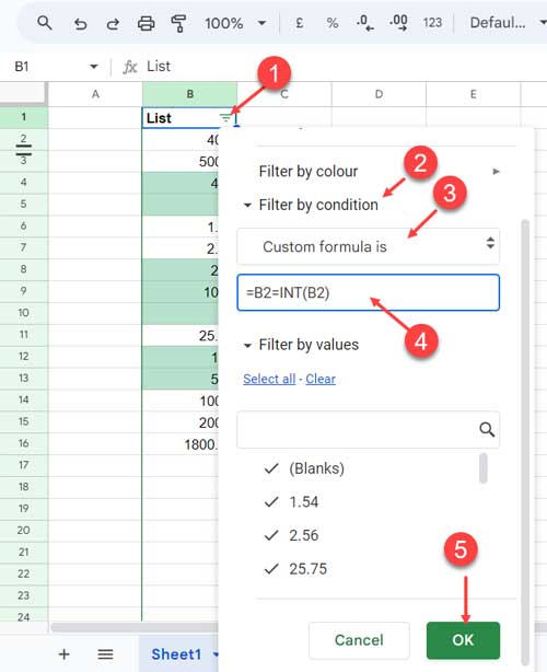
This will filter only whole numbers in the list.
FILTER Function vs. FILTER Menu for Filtering Integers in Google Sheets
Here are two main points to consider when choosing between the two methods for filtering whole numbers:
- FILTER menu command:
- The Create a filter menu modifies the source list directly.
- When you add more values to the filtered range, you need to refresh the filter by clicking the filter icon in the first cell of the range and then clicking OK.
- FILTER function:
- The
FILTERfunction filters integers into a new range. - When you add more values, the formula will automatically include them if the range is open (e.g.,
B2:Binstead ofB2:B16).
- The
I hope this helps you choose the method you want to use for filtering whole numbers in Google Sheets.
Conditional Formatting to Highlight Integers
To highlight integers in the range B2:B, you can use the following custom formula rule in Conditional Formatting in Google Sheets:
=AND(B2 > 0, B2 = INT(B2))Here is how to apply it:
- Go to Format > Conditional formatting.
- In the Apply to range field, enter the range
B2:BorB2:B16. - In the Format rules section, select Custom formula is.
- In the custom formula field, enter the formula above.
- Click Done.
We have learned how to use the FILTER function as well as highlight integers in Google Sheets. The next tip is how to mark them.
How to Mark or Extract Whole Numbers
In some cases, you may need to mark the rows that contain whole numbers.
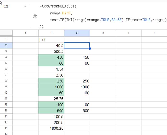
In our case, the range is B2:B. We can use the following ARRAYFORMULA in row 2 of any blank column in that sheet:
=ARRAYFORMULA(
   LET(
        range, B2:B,
        test, IF(INT(range) = range, TRUE, FALSE), IF(range = "",, test)
   )
)
It is recommended to enter this formula in cell C2. It will return TRUE for integers and FALSE for decimals. You can replace TRUE and FALSE in the formula with any custom values, such as 1 for TRUE and 0 for FALSE.
If you want to extract only the integers, replace the logical test IF(range = "",, test) with IF(test = TRUE, range). Here is the corrected formula:
=ARRAYFORMULA(
   LET(
        range, B2:B,
        test, IF(INT(range) = range, TRUE, FALSE), IF(test = TRUE, range,)
   )
)
Anatomy of the Formula
The formula can also be simplified to:
=ARRAYFORMULA(IF(INT(B2:B) = B2:B, TRUE, FALSE))The LET function is used to define names for expressions, enhancing performance.
The IF function works by first using the INT function to convert the value in each cell to an integer. Then, it compares the converted value to the original value. If the two values are equal, the formula returns TRUE; otherwise, it returns FALSE.
The ARRAYFORMULA function allows the formula to be applied to all the cells in the range, not just the active cell.


