How to Highlight N Columns Alternately in Google Sheets

Want to visually group columns in Google Sheets—for timelines, project phases, or budgeting categories? In this tutorial, you’ll learn how to highlight N columns alternatively in Google Sheets using conditional formatting.

This means highlighting blocks of columns (e.g., the first 2 columns), skipping the next N columns, then highlighting the next N, and so on.

You can customize the block size by setting N to any number of columns, and optionally control it from a cell.

Example of highlighting every alternate group of N columns in Google Sheets using conditional formatting

Table of Contents

Example: Highlight N Columns Alternately in Google Sheets

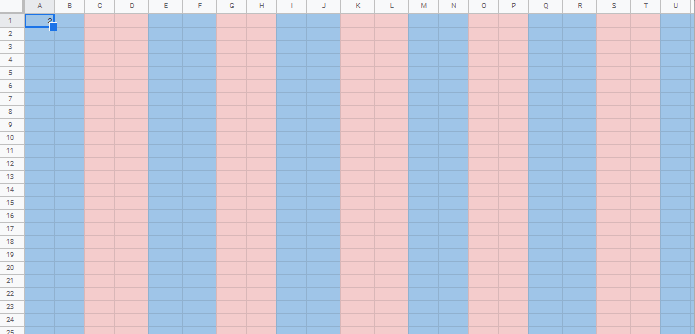
Let’s say N = 2. With the formulas provided below, columns A and B will be highlighted in light blue, C and D in light red, E and F in light blue again, and so on — creating a clear alternating pattern of column groups.

You can also make this behavior dynamic by referring to a cell (like A1) that holds the N value.

Conditional Formatting Formulas

Apply the following rules to a range like A1:Z1000. You can later adjust the range as needed.

Before applying the rule, enter the number of columns to group (N) in cell A1. For example, enter 2 to highlight every alternate set of 2 columns.

Rule #1 – Light Blue Background

=MOD(COLUMN(A1)-COLUMN($A$1), $A$1*2) < $A$1

Explanation:

This formula checks if the current column falls within the first N columns of each 2N group. It uses the MOD function to cycle through blocks of 2×N columns and highlight the first N in each block.

Rule #2 – Light Red Background (Optional)

=MOD(COLUMN(A1)-COLUMN($A$1), $A$1*2) >= $A$1

Explanation:

This highlights the alternate group — the second set of N columns in each 2N block. If you’re using two colors, apply this as a second rule.

Dynamic Control of N Using a Cell

In both formulas above, $A$1 refers to the cell where you can enter the value of N. This allows you to change the group size at any time.

A1 Value	Highlighting Pattern
1	Every other column (A, C, E, …)
2	Every alternate set of 2 columns (A–B, E–F, …)
3	Every alternate set of 3 columns (A–C, G–I, …)
…	And so on

To make the formatting static (non-dynamic), simply replace $A$1 in the formulas with a number (e.g., 2 or 3).

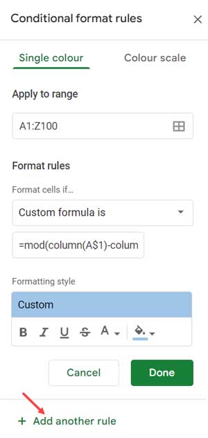
How to Apply the Conditional Formatting Rules

Follow these steps to set up the alternating group highlighting in Google Sheets:

Select the range — for example, A1:Z1000.
Go to Format > Conditional formatting.
Under Format cells if, choose Custom formula is.
Paste the Rule #1 formula and choose a fill color (e.g., light blue).
Click Add another rule.
Paste the Rule #2 formula and choose a second fill color (e.g., light red).
Click Done.
In cell A1, enter the desired block size — try entering 3 and observe the alternating column highlights.

Conditional formatting rule settings to highlight N columns alternatively in Google Sheets

Highlight N Columns Alternately Starting From a Different Column

You might want to skip certain starting columns like A to C and begin the formatting from column D instead.

To do that, use the formulas below:

Light Blue:

=MOD(COLUMN(D1)-COLUMN($D$1), $A$1*2) < $A$1

Light Red:

=MOD(COLUMN(D1)-COLUMN($D$1), $A$1*2) >= $A$1

Apply these formulas to the range D1:Z1000.
Then enter 5 in cell A1 to highlight every other block of 5 columns starting from column D.

Wrapping Up

Now you know how to highlight N columns alternatively in Google Sheets, whether starting from column A or a different column. This method is flexible, dynamic, and visually helpful for separating data into groups.

How to Highlight Groups of N Columns Alternately in Google Sheets