When working with drop-down lists in Google Sheets, it’s common to encounter invalid entries—values typed or pasted that aren’t part of your allowed list. Identifying these entries helps maintain data quality.
By default, Google Sheets shows a small error flag (a red triangle) in the corner of any cell containing an invalid entry, which helps you spot them. However, these flags can be easy to miss, especially in large sheets. That’s why highlighting invalid entries with color or other formatting can make them much more visible and easier to manage.
Google Sheets offers two ways to create drop-down lists:
- From a range — where list items come dynamically from a range of cells.
- Manually entered list — where options are typed directly into the data validation settings.
Depending on the type, you can highlight invalid entries using either a formula with conditional formatting or a simple Apps Script. This guide covers both methods.
1. Highlight Invalid Entries in Drop-down Lists from a Range
Assume you have a list of fruits in Sheet2 column A:
Apple
Orange
Mango
Banana
To create a drop-down in Sheet1 column A using this list:
- Select cell
A2inSheet1. - Click Insert > Drop-down.
- Choose Drop-down (from a range) in the sidebar.
- Select
Sheet2!A1:Aas the range.
- Under Advanced options, select Show a warning.
- Click Done.
You can copy the drop-down down the column (e.g., A3:A10).
If a user enters a value like “Avocado” (not in the list), Google Sheets will display a warning icon. However, these warnings are easy to overlook.

Highlight Invalid Entries with Conditional Formatting
To make invalid entries stand out:
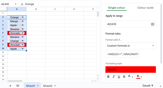
- Select the drop-down range (e.g.,
A2:A10). - Go to Format > Conditional formatting.
- Under Format rules, select Custom formula is.
- Enter the following formula:
=AND(A2<>"", ISNA(XMATCH(A2, INDIRECT("Sheet2!A1:A")))) - Choose a fill color (red is recommended).
- Click Done.
Cells with values not in the original list will now be highlighted in red.
2. Highlight Invalid Entries in Manually Created Drop-down Lists
If you create drop-down lists by typing options directly:
- Select cell
B2inSheet1. - Click Insert > Drop-down.
- Manually enter options such as Apple, Orange, Mango, Banana.
- Under Advanced options, select Show a warning.
- Click Done.
- Copy the drop-down down the column (e.g.,
B3:B10).
Entering an invalid value like “Avocado” will show a warning but will not be visually highlighted.
Highlight Invalid Entries with Apps Script
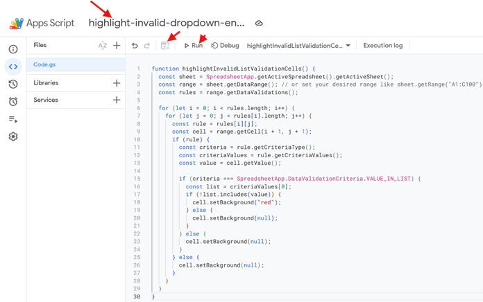
The following script highlights cells in red where the value is not part of the manually defined drop-down list:
function highlightInvalidListValidationCells() {
  const sheet = SpreadsheetApp.getActiveSpreadsheet().getActiveSheet();
  const range = sheet.getDataRange(); // or set your desired range like sheet.getRange("A1:C100")
  const rules = range.getDataValidations();

  for (let i = 0; i < rules.length; i++) {
    for (let j = 0; j < rules[i].length; j++) {
      const rule = rules[i][j];
      const cell = range.getCell(i + 1, j + 1);
      if (rule) {
        const criteria = rule.getCriteriaType();
        const criteriaValues = rule.getCriteriaValues();
        const value = cell.getValue();

        if (criteria === SpreadsheetApp.DataValidationCriteria.VALUE_IN_LIST) {
          const list = criteriaValues[0];
          if (!list.includes(value)) {
            cell.setBackground("red");
          } else {
            cell.setBackground(null);
          }
        } else {
          cell.setBackground(null);
        }
      } else {
        cell.setBackground(null);
      }
    }
  }
}
How to use the script:
- Open your Google Sheet.
- Navigate to Extensions > Apps Script.
- Remove any existing code and paste the above script.
- Rename the file by clicking on “Untitled project” at the top and entering “highlight-invalid-dropdown-entries”.
- Save the project.
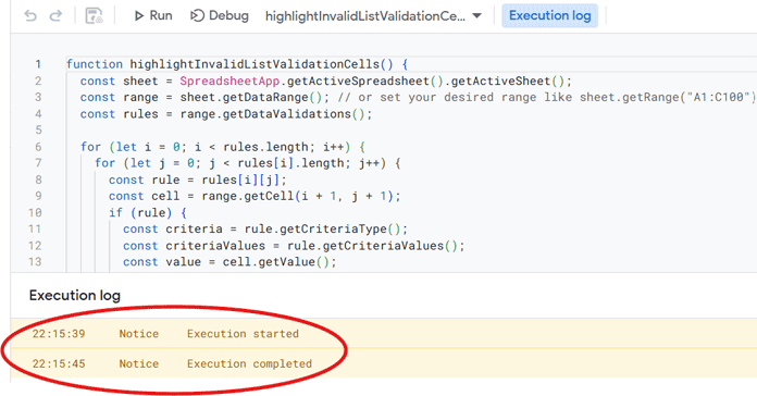
- Click the run ▶️ button.
- Authorize the script when prompted.
- The script will highlight invalid entries in the active sheet.
Pros and Cons of Each Method
| Method | Pros | Cons |
|---|---|---|
| Drop-down from range + formula | Easy to set up and automatically updates if the list changes. | Works only on the selected range; if applied broadly, it may highlight cells without data validation, causing false positives since it checks value presence, not validation rules. |
| Manually entered drop-down + script | Specifically checks cells with data validation rules, can scan any range or entire active sheet, and works with multiple drop-downs having different lists. | Requires Apps Script knowledge and manual script execution; initial setup takes more effort. |
| Both | Helps maintain data integrity and highlights invalid entries clearly. | Each method has its limitations; combining both may be needed for complete coverage. |
Note on Preventing Invalid Entries
You can avoid invalid entries altogether by selecting Reject input in the drop-down’s Advanced options. This setting prevents users from entering anything outside the list, eliminating the need for highlighting or scripts.
Conclusion
Highlighting invalid entries improves data integrity and makes errors easy to spot. Use conditional formatting with XMATCH for range-based drop-downs and the Apps Script for manually entered lists.
This tutorial is part of The Ultimate Guide to Conditional Formatting in Google Sheets, where you’ll find 80+ practical conditional formatting techniques.


