Google Sheets: Adaptive Study Planner with Auto-Reschedule

Below is a free download link to an adaptive study planner template for use in Google Sheets, along with instructions on how to use it.

This adaptive study planner template helps you effectively schedule and manage your study sessions for each chapter.

First, enter the initial study date of a chapter. Then, input your spaced repetition intervals for the second, third, and subsequent revisions of that chapter. In another column, enter the actual completion date. With each completion date, the next revision date will be calculated automatically. Continue this process with other chapters.

The number of revisions needed to effectively memorize a chapter can vary depending on the complexity of the material and individual learning styles. You are free to modify the spaced repetition intervals to suit your needs, and I’ll explain how to do that as well.

Download the Adaptive Study Planner Template

Adjusting the Spaced Repetition Settings

Spaced repetition refers to the interval after which you should revise a chapter.

1 = After 1 day
2 = After 2 days
…
60 = After 60 days

You can find these spaced repetition intervals in the range D2:M2, and their corresponding serial numbers in D1:M1. You can modify the values in D2:M2 according to your needs.

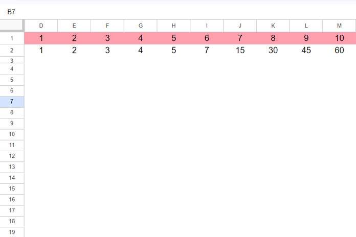
Adjusting the Spaced Repetition Settings

We will use the serial numbers as the input within the template. For example, if you want to start a revision after 15 days, you should specify 7, which is the serial number for 15.

Note: The template currently supports ten-spaced repetitions. If you want to add more, you can enter them in N1:S1 and N2:S2. You’ll also need to modify the ranges $D$1:$M$1 and $D$2:$M$2 in the formulas in cells C7, F7, I7, L7, O7, and R7 accordingly.

Using the Adaptive Study Planner

The template is currently set up for 6 chapters, with each chapter having three columns. You can add more chapters if needed, which I’ll explain as well.

Planning the Study of the First Chapter:

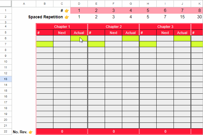
Overview of the Adaptive Study Planner Template in Google Sheets

In the third column, enter the initial study date for the chapter in the dark yellow highlighted cell (e.g., cell D6).
In cell B7, highlighted in dark yellow, enter the serial number corresponding to your desired spaced repetition interval. For example, if you want to revise the chapter after 45 days, enter 9.
In cells B8, B9, B10, etc., enter the serial numbers for the third, fourth, fifth, and subsequent spaced repetitions.
You will get the second revision date in C7. Enter it in D7 to get the next completion date in C8. Enter it in D8, and continue this process until you have completed all the revision dates.

You can follow the same steps for the other chapters.

Important:

When you complete a revision according to the schedule, you do not need to make any changes. However, if any revision completion date in column D differs from the schedule in column C, update the date in column D. Then, adjust the dates of subsequent revision completions in column D based on the refreshed dates in column C.

Note: Do not make any changes to the second column in each chapter, as it is dedicated to formulas. These formulas help automatically reschedule the study planner.

Adding Chapters and Revisions

The template currently supports 6 chapters. If you want to add a 7th chapter:

Copy the range Q4:S22.
Navigate to cell T4 and paste the copied range.
Delete any contents in the first and last columns.

The template currently supports up to 15 revisions. If you want to add more:

Select row #20, right-click, and select “Insert 1 Row Below.”

Adaptive Study Planner Formula and Explanation

You can skip this part as it only covers the formulas and a brief explanation.

Under each chapter, the first and second cells in the second column contain formulas.

Chapter 1 Formula #1 (Cell C6):

=D6

This formula in cell C6 copies the initial study date. You won’t see the result in cell C6 since the font color matches the background. The following formula in cell C7 uses this value.

Chapter 1 Formula #2 (Cell C7):

=ArrayFormula(
   LET(
      rev_grade, B$7:B$21, 
      rept, $D$2:$M$2, 
      reptiD, $D$1:$M$1, 
      rev_first, C$6, 
      test, 
         IFNA(MAP(
            rev_grade, SEQUENCE(ROWS(rev_grade)), 
            LAMBDA(valA, valB, 
               OFFSET(rev_first, valB-1, 1)+
               XLOOKUP(valA, reptID, rept)
            )
         )), 
      IF(test>15, test,"")
   )
)

Where:

$D$2:$M$2 = The spaced repetition intervals.
$D$1:$M$1 = The serial numbers of the spaced repetition intervals.
B$7:B$21 = The user-entered spaced repetition serial numbers.
C$6 = The reference containing the initial study date entry copied from cell D6.

Formula Explanation:

OFFSET(rev_first, valB-1, 1): This formula in cell C7 offsets 0 rows and 1 column from C6 to get the date from D6.
XLOOKUP(valA, reptID, rept): Returns the spaced repetition interval based on the user input in B7.

The formula adds the XLOOKUP output to the OFFSET output to calculate the next revision date in C7. Since this formula is used as a custom function with MAP LAMBDA, it repeats in each row. The OFFSET formula increments the row number (0, 1, …), while the XLOOKUP searches for the current row element in column B within the spaced repetition serial numbers and retrieves the corresponding spaced repetition interval.

Fix Fractional Percentage Formatting Issues in Google Sheets

Lookup the Smallest Value in a 2D Array in Google Sheets