The DGET function is the only database function in Google Sheets that can perform a vertical lookup within a structured dataset. While most database functions in Sheets focus on aggregation, DGET stands out for retrieving values from a specific column, similar to a vertical lookup. It can return values from multiple columns but not rows.
To use the DGET function effectively, ensure that your dataset meets the following basic database requirements:
- The data should be structured in tabular form, with the top row containing field labels.
- There should be no duplicate entries in the lookup column (criteria field). If duplicates exist, use functions like UNIQUE or SORTN to remove them before applying DGET. This is important because DGET will return an error if multiple matches are found.
- Ensure there are no merged cells within the data range.
In summary, DGET works best with well-structured datasets that are free from duplicates and merged cells.
DGET Function: Syntax and Basic Example
Syntax:
DGET(database, field, criteria)This syntax is common to all database functions in Google Sheets, such as DSUM, DPRODUCT, DCOUNT, etc. Only the function name differs.
Details about the Function Arguments:
You don’t need to focus heavily on the arguments; you can learn the usage of the DGET function in Google Sheets from the examples provided.
database: This is the array or range containing the data to consider. It should meet the three conditions mentioned earlier in the tutorial.field: The field represents the column label or column number where the values are extracted. You can compare the field in DGET to the index number in VLOOKUP.criteria: The criteria are an array or range containing one or more conditions used to filter the database. In VLOOKUP terms, criteria in the DGET function serve as search keys.
Understanding the Usage
Here’s a basic example of how to use the DGET function in Google Sheets.
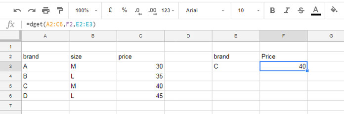
The sample data includes the field labels ‘brand’, ‘size’, and ‘price’ in A2:C2, with relevant data below in A3:C6.

Let’s look up the brand “C” in the first column and return the price from the third column. Follow these steps:
- Criteria: Enter “brand” in E2 and “C” in E3 (lookup column label and value).
- Field: Enter “price” in F2.
Now, use the following DGET formula:
=DGET(A2:C6, F2, E2:E3)Specifying the criteria and field as cell references is straightforward in DGET. You can also hardcode them:
=DGET(A2:C6, "price", {"brand"; "C"})Alternatively, you can replace the field label with the column number:
=DGET(A2:C6, 3, {"brand"; "C"})How to Extract Multiple Column Values Using DGET in Google Sheets
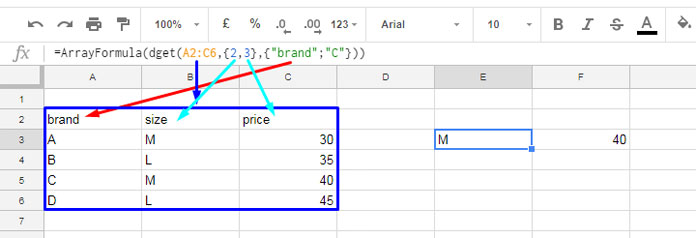
To extract multiple values, specify the field numbers as an array constant within the DGET function. Here’s an example:
=ArrayFormula(DGET(A2:C6, {2, 3}, {"brand"; "C"}))This formula searches for the key “C” in the “brand” column and returns the values from the second and third columns in the range A2:C6.

The DGET function is designed to return a single output. To return more than one value, you should use the ARRAYFORMULA function alongside it.
How to Use Multiple Criteria in DGET in Google Sheets
Like other database functions in Google Sheets, you can easily apply multiple criteria in DGET when using cell references for the criteria.
For example, to search for the brand “C” and size “M”, you can enter them in a range and refer to that range in your formula. The criteria range should look as follows:
| brand | size |
| C | M |
Alternatively, you can hardcode the criteria as follows:
=ArrayFormula(DGET(A2:C6, 3, {"brand", "size"; "C", "M"}))Pros and Cons of the DGET Function in Google Sheets
Pros:
- Easy to use and specify criteria (lookup values).
- Offers better performance compared to other lookup functions.
- Not restricted to lookups in the first column, unlike VLOOKUP.
- Supports partial matches by default. For example, “A” will match “A” and “ABC”. For exact matches, place an equal sign in front of the criterion. Please see the “Resources” section below.
Cons:
- Requires structured data.
- Multiple occurrences of search keys in the lookup column cause errors.
- Does not support approximate matches for numeric or date criteria.


Hi Prashanth,
Is there a way to use DGET to continue to run down a column as data continues to come in?
I need this to run continuously:
=DGET('Settlement Data'!$A$1:$H,"Revenue",{"WE","Ranch","Program";N3,O3,P3})I tried this but I get an error for more than one match found:
=ArrayFormula(if(isblank(N3:N),"",DGET('Settlement Data'!$A$1:$H,"Revenue",{"WE","Ranch","Program";N3:N,O3:O,P3:P})))Any Ideas?
Hi, Chris,
Please see if this tutorial helps?
DGET Array Formula to Run Down a Column in Google Sheets.
Hi Prasanth,
Thanks. It works.
Hi Prashanth,
I need to get the Database in Sheet1 (UPC, Item No., Price).
In Sheet2, I have to match the database items and get item no. Sheet 2 having (Upc, Product Description).
But the thing is, the sheet2 UPC is comma-separated values given. Need to extract the UPC and match it with Sheet1 UPC. I get the Individual UPC and match it with INDEX & MATCH function. But I could not able to get the comma-separated UPC in Sheet 2.
I request you to kindly give a solution to get this done.
It will very helpful.
Hi, Saravanan,
In Sheet2!C2 (as Sheet2!A1:C1 may contain field labels), enter the following formula and drag-down.
=textjoin(", ",true,iferror(ArrayFormula(vlookup(trim(split(A2,",")),Sheet1!$A$1:$B$5,2,0))))Thanks, Prasanth for your quick response. I used this in google sheet. But I get #N/A. For your reference, I shared the google sheet for your kind reference. Please look and give the solution to fix.
Hi, Saravanan,
Updated your sheet with my formula.
You have missed a comma after the TRUE argument in the TEXTJOIN part.
Further, I have converted the split text values back to numeric using the VALUE function.
Seems, it works now!
I was recently confronted with a problem.
Where “B-BOX” and “B-BOX PRO” are considered duplicates in this formula.
Is there a way to resolve this?
Hi, Jason,
I have addressed the aforesaid DGET problem in my tutorial below.
Exact Match in Database Functions in Google Sheets – How-To
Contrary to the Con #2, it is actually possible to use multiple criteria in the Sheets database functions such as DGET, separated by a semicolon.
Syntax examples:
=DGET(database,"field",TRANSPOSE({"Country","Switzerland";"City","Zurich"}))=DGET(database,"field",TRANSPOSE({"Country","Switzerland","Switzerland";"City","Zurich","Geneva"}))Hi, Jan,
Thanks for pointing out the mistake!
I was aware of how to use the multiple criteria as a cell reference in Dget. But new to the use of criteria within formula as you have pointed out at least at the time of writing this post (a few months back).
Updated the post and given due credit to you.
Have a nice day!