


")


")

")
")
 in Excel & Google Sheets")


This tutorial will discuss a powerful technique for filtering rows with formula errors in Google Sheets.
We will create a custom formula that works seamlessly within the filter criteria of any column in your filtered range or table.
This formula effectively identifies errors present in any column across all rows, regardless of your chosen filter column.
This will allow you to quickly identify and address these problematic rows in your data, which is crucial for troubleshooting and data cleaning in large datasets.
Creating a Flexible Formula for Formula Error Filtering
We will primarily use two functions, ERROR.TYPE and XMATCH, to filter formula errors in rows within a range or table in Google Sheets. Since this will be an array formula, the ARRAYFORMULA function is also required.
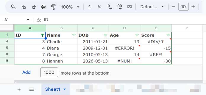
My sample data is in A1:E, where I intentionally placed different types of errors in columns to experiment with filtering. In that data, A1:E1 contains field labels.
Formula to Filter Error Rows in Google Sheets
=ArrayFormula(XMATCH(1, ERROR.TYPE($A2:$E2), 1))This formula can be used to filter rows with formula errors in the dataset. You’ll need to write the formula for the first record in your table, as demonstrated above. It will then be applied to the entire filter range.
Let’s apply this custom error filtering formula in the Filter, and we will start by creating the filter for completeness.
- Select A1:E.
- Click on Data > Create a filter.
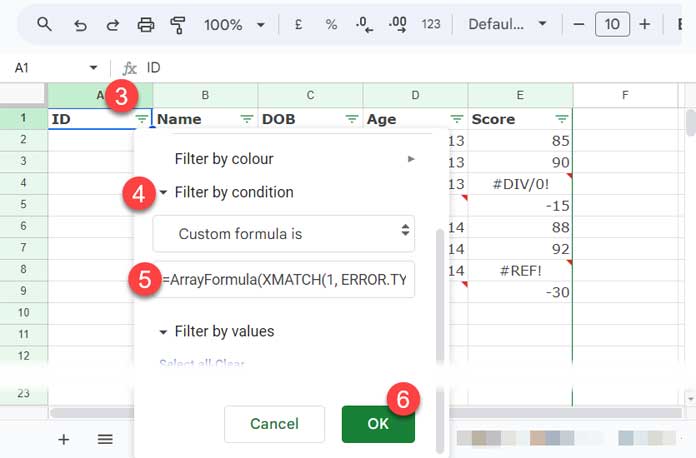
- Click the filter drop-down within the first column, i.e., A1, or any other column. The formula has no issue identifying errors across the row, irrespective of the column you choose.
- Click Filter by Condition and select “Custom formula is”.
- In the given field, copy-paste the above formula.
- Click OK.
This filters out all rows that don’t contain any errors. You will see only the error rows, allowing you to check each cell with errors and pinpoint the issue.
This is the best approach to filter error rows in Google Sheets.
Formula Breakdown
The formula is straightforward. Let me break it down for you.
Section 1:
=ArrayFormula(ERROR.TYPE($A2:$E2))The ERROR.TYPE function, following the syntax ERROR.TYPE(reference), returns a number corresponding to the error value or #N/A if there is no error. We used this across the row, so it requires the ARRAYFORMULA function.
The output will be an array equal in size to the specified range, containing error numbers (ranging from 1 to 8) or #N/A errors.
Section 2:
=ArrayFormula(XMATCH(1, ERROR.TYPE($A2:$E2), 1))Syntax: XMATCH(search_key, lookup_range, [match_mode], [search_mode])
Where:
search_key: 1lookup_range:ERROR.TYPE($A2:$E2)match_mode: 1
The XMATCH function searches for 1 (search_key) in the ERROR.TYPE output (lookup_range) and returns the relative position if it matches any cell in the array, or #N/A if it doesn’t.
The match_mode in XMATCH is 1, so it searches for the search key, and if not found, it returns the relative position of the next value greater than the search key. This ensures the formula can match any error numbers from 1 to 8.
The formula is coded for the first record. When applied within the filter, it extends to each row in the filtered area.
This formula filters out rows wherever XMATCH returns #N/A, resulting in visibility only for the rows that contain at least one formula error.
Create a Custom Filter for Specific Error Types (Advanced Tip)
The above formula filters rows with all types of formula errors. Do you want to target a specific type of formula error, such as #N/A?
You need to make just two changes in the formula. The search key in the XMATCH function must be one of the following error numbers corresponding to the error type, and the match mode must be 0, which is an exact match of the search key.
| Error Number | Error Value |
| 1 | #NULL! |
| 2 | #DIV/0! |
| 3 | #VALUE! |
| 4 | #REF! |
| 5 | #NAME? |
| 6 | #NUM! |
| 7 | #N/A |
| 8 | All other errors |
For example, to filter all rows containing the #N/A errors, use this formula.
=ArrayFormula(XMATCH(7, ERROR.TYPE($A2:$E2), 0))Where:
search_key: 7lookup_range:ERROR.TYPE($A2:$E2)match_mode: 0
Resources
The following tutorials will help you identify and troubleshoot some of the formula errors in Google Sheets.
- How to Highlight All Error Rows in Google Sheets
- Common Errors in Vlookup in Google Sheets
- Highlight Cells with Error Flags in the Drop-down in Google Sheets
- ARRAY_ROW Function #REF Error and Solution in Google Sheets
- IMPORTRANGE Result Too Large Error: Solution
- How to Remove #REF! Errors in Google Sheets (Even When IFERROR Fails)