You can filter a custom calendar with events in two ways in Google Sheets. One method retains the grid layout, while the other presents the data in a tabular form. We will explore both options.
A custom calendar in Sheets is mainly used to enter events, assignments, and retrieve data for specific days using formulas from other sheets.
How do you filter specific events or other data from this custom calendar while maintaining the grid layout or converting it into a tabular format?
Let’s explore both methods with examples.
Filter a Custom Calendar with Events While Keeping the Grid Layout
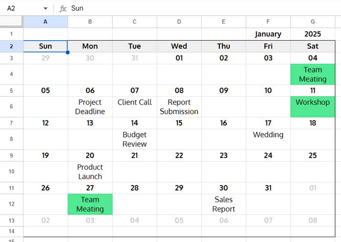
In the following example, I have created a custom calendar in the range A2:G14.

I want to filter this calendar for the events “Team Meeting” and “Workshop”.
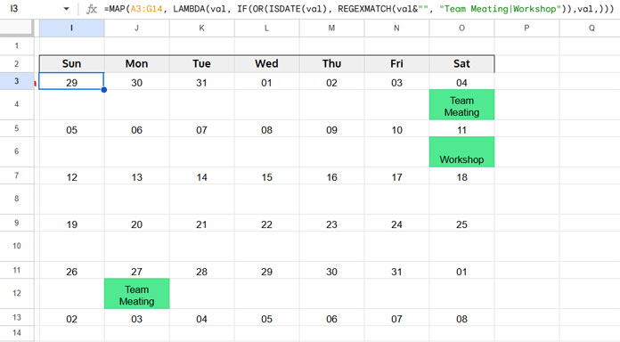
The goal is to copy the calendar to a new range while removing all other events. Here’s how to do it.
Enter the following formula in an empty cell. Ensure that it has enough space to expand; otherwise, it will return a #REF! error.
=MAP(A3:G14, LAMBDA(val, IF(OR(ISDATE(val), REGEXMATCH(val&"", "(?i)Team Meating|Workshop")),val,)))
This formula assumes you have used dates (not numbers) in the calendar. Dates may be formatted as two-digit values representing days, which is not an issue. However, if you have numbers instead of dates, replace ISDATE(val) with ISNUMBER(val).
To filter an additional event, include it in the regex pattern separated by a pipe (|), as shown below:
"(?i)Team Meating|Workshop|Client Call"This way, you can add more conditions to the filter.
Note: When using ISDATE, the formula filters all dates in the calendar. If you enter dates in the event row, they will be filtered as well. To prevent this, enter them as text by prefixing them with an apostrophe ('). Similarly, when using ISNUMBER, it will extract both dates and numbers in event rows. To avoid this, enter numeric values as text, also by starting them with an apostrophe (').
How This Formula Filters the Custom Calendar While Keeping the Grid Layout
Here’s a breakdown of how the formula works:
- The MAP function applies a custom LAMBDA function to each value in the range, producing a new array.
- The LAMBDA function evaluates whether the current value is a valid date or one of the specified events.
LAMBDA(val, IF(OR(ISDATE(val), REGEXMATCH(val&"", "(?i)Team Meating|Workshop")),val,)) - If TRUE, it returns the value; otherwise, it returns a blank cell.
- MAP processes each element in the calendar range, filtering only the specified dates and events while keeping the original layout.
This approach maintains the calendar’s structure. But what if you want to filter events and their corresponding dates into a tabular format? Let’s explore that next.
Filter a Custom Calendar with Events into a Tabular Format
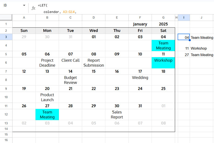
Use the following formula to filter a custom calendar for specific events and display them in a tabular format:
=LET(
   calendar, A3:G14,
   row_start, 3,
   height, 2,
   seq, SEQUENCE(ROWS(calendar)/height, 1, row_start, height),
   QUERY(REDUCE(TOCOL(,3), SEQUENCE(7), LAMBDA(acc, val, VSTACK(acc, HSTACK(FILTER(CHOOSECOLS(calendar, val), XMATCH(ROW(calendar), seq)), WRAPROWS(FILTER(CHOOSECOLS(calendar, val), NOT(IFNA(XMATCH(ROW(calendar), seq)))), height-1))))), "Select * where lower(Col2) matches 'team meating|workshop' order by Col1",0)
)
Explanation of the Formula
A3:G14represents the calendar range, starting from the first row with dates to the last row with events.row_startdefines the row where the first week’s dates begin (row3in this case).heightspecifies the number of rows per week (including the date row and event row). This value must remain consistent across all weeks. In our case, it is2.- QUERY filters the events based on the specified conditions (
'team meeting|workshop'). You can add more conditions by separating them with pipes (|)
Formula Breakdown
This formula is based on a method I previously shared in my post titled “Convert Google Sheets Calendar into a Table.”
I have modified that formula to include filtering. Here’s the key part:
QUERY(REDUCE(TOCOL(,3), SEQUENCE(7), LAMBDA(acc, val, VSTACK(acc, HSTACK(FILTER(CHOOSECOLS(calendar, val), XMATCH(ROW(calendar), seq)), WRAPROWS(FILTER(CHOOSECOLS(calendar, val), NOT(IFNA(XMATCH(ROW(calendar), seq)))), height-1))))), "Select * where lower(Col2) matches 'team meeting|workshop' order by Col1", 0)The original formula structured the calendar data into a table. By adding QUERY, we now filter the tabular output based on the specified events.
Regarding filtering, we used the MATCHES regular expression to match multiple conditions at once. Since it is case-sensitive, specify the criteria in lowercase letters. We convert all event data to lowercase (lower(Col2)) before comparison.
Note: The height in the above calendar is 2, meaning one date row followed by one event row. This results in two columns (date and event). If the height is 3 (one date row followed by two event rows), the output will have three columns. This may cause issues in filtering if you are not familiar with QUERY. To keep it simple, use one event row. If you require two event rows, modify the formula as follows:
"Select * where lower(Col2) matches 'team meeting|workshop' or lower(Col3) matches 'team meeting|workshop' order by Col1"For a detailed explanation, check out my tutorial on converting a Google Sheets calendar into a table.
Resources
- Filter Today’s Events from a Calendar Layout in Google Sheets
- Hyperlink Calendar Dates to Events in Google Sheets
- How to Count Events in Particular Time Slots in Google Sheets
- Calendar View in Google Sheets (Custom Template)
- Dynamic Yearly Calendar Template in Google Sheets: Free Template and How-To Guide
- Fully Flexible Fiscal Year Calendar in Google Sheets
- Create Monthly Calendars in Google Sheets (Single & Multi-Cell Formulas)


