In this tutorial, I’ll show you how to extract numbers from square brackets in Google Sheets. Whether your cell contains one or multiple bracketed numbers, you’ll find a reliable and easy-to-follow solution using formulas.

Extract Numbers Within Single Square Brackets

To extract numbers from square brackets when there’s only one set per cell, use the REGEXEXTRACT function:

Example:

Value in cell A1: Team A [200]

Formula:

=IFNA(VALUE(REGEXEXTRACT(A1, "\[([0-9.]+?)\]")))

Result: 200

Explanation:

• REGEXEXTRACT(A1, "\[([0-9.]+?)\]"): Extracts the number inside the first pair of square brackets. The regular expression \[([0-9.]+?)\] matches digits (including decimals) enclosed in brackets.
• VALUE(...): Converts the extracted text into a numeric value.
• IFNA(...): Returns a blank if no number is found, avoiding a #N/A error.

This formula is perfect when you only need to extract the first number from square brackets in each cell.

Apply the Formula to a Column Range

Yes, you can apply this formula to a column range using ARRAYFORMULA:

=ArrayFormula(IFNA(VALUE(REGEXEXTRACT(A1:A10, "\[([0-9.]+?)\]"))))

This extracts the first number found in square brackets from each cell in the range A1:A10.

Extract Numbers from Multiple Square Brackets in a Cell

If a cell contains multiple numbers in square brackets, the previous method only extracts the first one. Here’s a formula that extracts all such numbers:

Example:

Value in cell A1: Lap 1 [200.5] Lap 2 [195.25]

Formula:

=ArrayFormula(IFERROR(VALUE(TOROW(IFERROR(REGEXEXTRACT(SPLIT(A1, "["), "^([0-9.]+?)\]")), 3))))

Result:

200.5
195.25

Step-by-Step Breakdown:

1. SPLIT(A1, "[")
   Splits the text at every opening square bracket [.
   Result:
   {"Lap 1 ", "200.5] Lap 2 ", "195.25]"}
2. REGEXEXTRACT(..., "^([0-9.]+?)\]")
   Extracts numbers that appear at the start of each split part, up to the closing bracket.
3. IFERROR(...)
   Handles any errors caused by segments that don’t contain valid numbers.
4. TOROW(..., 3)
   Converts the column of results into a single row and removes blanks.
5. VALUE(...)
   Converts text such as "200.5" into the numeric value 200.5.
6. Outer IFERROR(...)
   Ensures the formula still works if nothing is extracted.

This method is ideal when you need to extract multiple numbers from square brackets in a single cell.

Extract Numbers from Square Brackets in an Array of Cells

Wrapping the previous formula directly in an ARRAYFORMULA won’t work due to the use of TOROW, which isn’t compatible with array input ranges.

To handle a range (e.g., A1:A10), use the MAP and LAMBDA functions to apply the logic to each row individually:

=MAP(A1:A10, LAMBDA(text, ArrayFormula(IFERROR(VALUE(TOROW(IFERROR(REGEXEXTRACT(SPLIT(text, "["), "^([0-9.]+?)\]")), 3))))))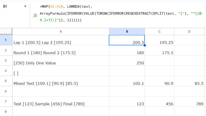

This formula extracts numbers from square brackets in each row of the range A1:A10, returning them as individual numeric arrays.

Resources

Here are more useful tutorials for working with text and numbers in Google Sheets:

• How to Extract Numbers from Text in Excel with Regex
• Extract All Numbers from Text and Sum Them in Google Sheets
• Extract, Replace, Match Nth Occurrence of a String or Number in Google Sheets
• Extract Numbers Prefixed by Currency Signs from a String in Google Sheets
• Extracting Numbers Excluding Dates from a Range in Google Sheets
• How to Extract Decimal Part of a Number in Google Sheets
• How to Extract Negative Numbers from Text Strings in Google Sheets