How to Extract Multiple Words Using REGEXEXTRACT in Google Sheets

We can use the REGEXEXTRACT function in Google Sheets to extract multiple words from a cell and put them into a row or column.

I don’t think it’s necessary to explain the purpose of this text extraction, as it varies depending on your job. However, here’s an example of a scenario where it might be useful.

I want to search a cell containing a list of country names and extract some of the countries if they exist in the list.

These are the names of some of the top countries where the blog Info Inspired has a good presence.

With the help of the REGEXEXTRACT function, I am extracting all of the matching words in a sentence, or comma-separated list, in a cell in Google Sheets.

We can use nested REGEXEXTRACT formulas (as shown in Figure 1 below) or a LAMBDA-based REGEXEXTRACT function (as shown in Figure 3 at the bottom) for this.

extract multiple matching words in a cell — Figure 1

Nested formulas are not ideal in all cases because they can make the formula lengthier and more difficult to understand. So, you would definitely want to try the LAMBDA-based formula instead.

Steps to Extract Multiple Words Using REGEXEXTRACT in Google Sheets

Syntax of the REGEXEXTRACT Function:

REGEXEXTRACT(text, regular_expression)

You can extract a single word from a cell by using the REGEXEXTRACT formula. For example, suppose cell A1 has the following country list:

India, United States, United Kingdom, Canada, Philippines, Australia, France, Brazil, Netherlands, Malaysia, Germany, Indonesia, Pakistan, South Africa, Spain, Singapore, Italy, Mexico, Sweden, Peru, Israel, Hong Kong, Vietnam, Bangladesh, Nigeria

If you want to extract the country name “Hong Kong,” you can use the following formula:

=REGEXEXTRACT(A1,"(?i)Hong Kong")

But don’t just stop there! You can make this REGEX formula behave like a logical test.

That means you can test cell A1 for the word “Hong Kong” and return the word if it is found, or else return another value.

This type of test is necessary. Otherwise, the REGEXEXTRACT function would sometimes return a #NA error.

Here is that formula, where we are making use of the IFERROR function:

=IFERROR(REGEXEXTRACT(A1,"(?i)Hong Kong"),"Not Available")

So, always remember to use the IFERROR function or the IFNA function together with REGEX in such scenarios.

Now, let us go back to our topic, which is how to extract multiple words using REGEXEXTRACT in Google Sheets.

Here, we can follow two approaches. If the number of words to extract is limited to 2-3 words, we can use a nested REGEXEXTRACT formula or a LAMBDA-based formula.

1. Nested REGEXEXTRACT Formula

The following formula extracts multiple words using REGEXEXTRACT in nested form, and the functions are separated by commas and placed within Curly Braces.

=IFERROR(
     {
     REGEXEXTRACT(A1,"(?i)Singapore"),
     REGEXEXTRACT(A1,"(?i)Italy"),
     REGEXEXTRACT(A1,"(?i)Brazil")
     }
)

The result would be as follows.

result showing multiple regex extract as an array — Figure 2

If the formula finds any mismatch, the result will have one or more blank cells.

For example, if cell A1 does not contain the word “Italy”, then cell D1 will be blank.

In our main formula (please refer to Figure 1 above), I have simply used the TRANSPOSE function to return the output into a column.

=TRANSPOSE(
     IFERROR(
          {
          REGEXEXTRACT(A1,"(?i)Singapore"),
          REGEXEXTRACT(A1,"(?i)Italy"),
          REGEXEXTRACT(A1,"(?i)Brazil")
          }
     )
)

You can use the QUERY function to remove blank cells and limit the number of values to a specific number (n).

=QUERY(
     TRANSPOSE(
          IFERROR(
               {
               REGEXEXTRACT(A1,"(?i)Singapore"),
               REGEXEXTRACT(A1,"(?i)Italy"),
               REGEXEXTRACT(A1,"(?i)Brazil")
               }
          )
     ),
"Select * where Col1<>'' Limit 3"
)

Here, the LIMIT clause in the last part controls the number of items to be returned. It’s 3 in the above formula.

2. Extract Multiple Words from a Cell in Google Sheets Using Lambda-Based REGEXEXTRACT

Syntax of the MAP Function:

MAP(array1, [array2, …], lambda)

If you want to extract a large number of matching words from a cell, you cannot use the nested REGEXEXTRACT formula in Google Sheets. The formula will become too large and difficult to manage.

Instead, you can use a MAP (LAMBDA helper function) and REGEXEXTRACT combo. This will allow you to extract multiple matching words without having to create a large and complex formula.

=LET(
     range,A1,
     value,{"Singapore","Italy","Brazil"},
     TOCOL(
          MAP(
               TOCOL(value,1),
               LAMBDA(r,REGEXEXTRACT(TEXTJOIN(" ",TRUE,range),"(?i)"&r))
          ),3
     )
)

Where:

Cell A1 contains the list of words to extract.
The array {"Singapore", "Italy", "Brazil"} contains the countries (values) to match in the list.

To match more values, you can insert them within the array (Curly Brackets) separated by commas.

This formula is flexible enough to:

Use a cell range like A1:A instead of a single cell like A1.
Match more values by placing them as a cell range like C1:C instead of a literal array, i.e., {"Singapore", "Italy", "Brazil"}.

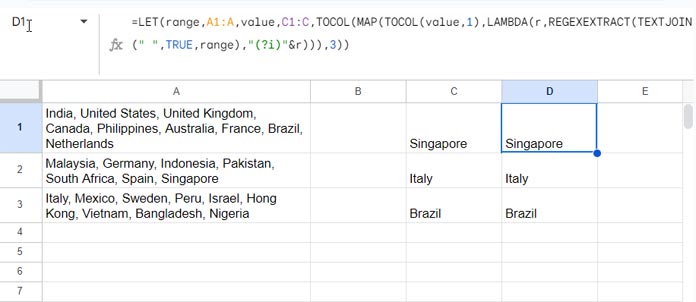
Here is an example:

=LET(
     range,A1:A,
     value,C1:C,
     TOCOL(
          MAP(
               TOCOL(value,1),
               LAMBDA(r,REGEXEXTRACT(TEXTJOIN(" ",TRUE,range),"(?i)"&r)
          )
     ),3
     )
)

Extract Multiple Words in Google Sheets Using Lambda-Based REGEXEXTRACT — Figure 3

That’s all I have to say about how to extract multiple words using REGEXEXTRACT in Google Sheets.

17 COMMENTS

Frank September 29, 2023 At 12:05 am

Hi Prashanth,

What if we needed to extract multiple or all occurrences of given patterns?

For example, consider these three patterns:

REGEXEXTRACT(A1:A,"(?i)($.*?$)"), REGEXEXTRACT(A1:A,"(?i)(\[.*?\])"), REGEXEXTRACT(A1:A,"(?i)(Cf\.\s.*?\.(\s|$))")

I tried the following formula, but it only extracts the first occurrence of each pattern:

=ArrayFormula(IF(REGEXMATCH(A1:A, "See Below"), "", IFERROR({ REGEXEXTRACT(A1:A, "(?i)($.*?$)"), REGEXEXTRACT(A1:A, "(?i)(\[.*?\])"), REGEXEXTRACT(A1:A, "(?i)(Cf\.s.*?\.(\s|$))") })))

- Prashanth September 30, 2023 At 9:53 am
  
  Hi Frank,
  
  It seems that extracting multiple occurrences of GIVEN PATTERNS with regex is not possible.
  
  You can try the following formula for the value in cell A2.
  
  =LET(test,TOCOL(SPLIT( SUBSTITUTE(SUBSTITUTE(SUBSTITUTE(SUBSTITUTE(SUBSTITUTE(SUBSTITUTE(A2, "(","|("),")",")|"),"[","|["),"]","]|"),"Cf","|Cf"),"*. ","*.|"),"|")), JOIN(" ",FILTER(test,(LEFT(test,1)="(")+(LEFT(test,2)="Cf")+(LEFT(test,1)="["))))
  
  If you want to spill this formula down, you may need to use the MAP function as follows:
  
  =IFERROR(MAP(A2:A,LAMBDA(row,LET(test,TOCOL(SPLIT( SUBSTITUTE(SUBSTITUTE(SUBSTITUTE(SUBSTITUTE(SUBSTITUTE(SUBSTITUTE(row, "(","|("),")",")|"),"[","|["),"]","]|"),"Cf","|Cf"),"*. ","*.|"),"|")), JOIN(" ",FILTER(test,(LEFT(test,1)="(")+(LEFT(test,2)="Cf")+(LEFT(test,1)="[")))))))
  
Frank September 5, 2023 At 6:12 pm

Is there a fix for the error “Calculation limit was reached while trying to compute this formula”?

Using:

=LET(range,A27:A8269,value,B27:B212, MAP(range,LAMBDA(range,TOROW( MAP(TOCOL(value,1),LAMBDA(r,REGEXEXTRACT(range,"(?i)"&r))),3))))

- Prashanth September 5, 2023 At 7:39 pm
  
  That’s expected with such a large range and nested MAP or other Lambda functions. The only possible solution is to split the data into multiple sheets and try again.
  
Frank September 2, 2023 At 7:02 pm

Hi Prashanth,

It works great! Thank you!

And it’s all dynamic, as a bonus.

I’ll try to figure out how it works as soon as possible, with all those new functions.

Thanks again!

Frank September 2, 2023 At 2:01 pm

Thanks. Here is the expected output in Sheet1:

[URL removed by admin]

And your 2nd output in Sheet2:

[URL removed by admin]

- Prashanth September 2, 2023 At 3:06 pm
  
  Hi Frank,
  
  Thanks for sharing your sample sheet. I couldn’t enter my formula because I only have view access.
  
  I understand that you want to extract multiple values from A1:A matching values in B1:B. But place the extracted values in the corresponding row not as a whole list.
  
  This formula in C1 will match B1:B in A1 and extract the matching values in C1:1, then match B1:B in A2 and extract the matching values in C2:2 and so on.
  
  =LET(range,A1:A3,value,B1:B, MAP(range,LAMBDA(range,TOROW( MAP(TOCOL(value,1),LAMBDA(r,REGEXEXTRACT(range,"(?i)"&r))),3))))
  
  I hope this is helpful!
  
Frank September 1, 2023 At 8:02 pm

Did you receive my new response from yesterday?

- Prashanth September 2, 2023 At 10:34 am
  
  Yes, please share a sample sheet URL.
  
Frank August 29, 2023 At 11:50 pm

What if I have more than 100 words over 1000+ cells with multiple occurrences per cell (most between 2 and 6) to extract? Don’t you have a simpler way than hardcoding the words reference strings? How about a solution using cell references? And possibly using a range?

- Prashanth August 31, 2023 At 6:44 pm
  
  Hi Frank,
  
  Thanks for your response.
  
  At the time of writing this tutorial, I had no option to do that. We are now armed with the LAMBDA functions. So we can use MAP or BYROW for that. I’ve updated this post to include an example.
  
Vineet Choudhary August 16, 2022 At 4:55 pm

Hi,

I have one issue with REGEXEXTRACT. I want to match and extract the exact word.

If I use the below formula, it will display the result “Sing.” But I want it to return “NA” because your A1 cell “Sing” word is not there.

=regexextract(A1,"(?i)Sing")

So, how can we extract the exact match instead of the partial match?

Thanks & Regards,

Vineet

- Prashanth August 17, 2022 At 11:31 am
  
  Hi, Vineet Choudhary,
  
  See if this formula work.
  
  =regexextract(A1,"(?i)^Sing$")
  
Kyn March 2, 2022 At 2:12 am

For the final query function, is the syntax off? Because when I try and use it for myself, it leaves me with a parse error.

I’m not sure about the end with a quotation without a starting quotation.

- Prashanth March 4, 2022 At 9:57 am
  
  Hi, Kyn,
  
  You may please check once again!
  
Hima Bindu February 25, 2020 At 11:32 am

I do have the start time 10 PM and end time 2 AM. I need to extract only numbers and the required time duration.

Thanks in Advance.

- Prashanth February 25, 2020 At 2:33 pm
  
  Hi, Hima,
  
  Extracting numbers are easy using Regex. But it won’t help us to find the duration. I wish to see the Sheet (sample) to provide you a possible solution.

Appointment Schedule Template in Google Sheets

Creating Sequential Dates in Equally Merged Cells in Google Sheets

Interactive Random Task Assigner in Google Sheets

Google Sheets Bar and Column Chart with Target Coloring

Analyzing Column A Between Non-Adjacent Values in Column B: Google Sheets

Automatically Pre-fill Google Forms from Google Sheets: A Step-by-Step Guide

How to Set Up Google Docs Forms: A Comprehensive Guide

How to Insert Drop-downs in Google Docs Documents

How to Create a Table and Pin and Unpin Header Rows…

How to Use Section Break in Google Docs

How to Split a Table in Google Docs

How to Create First Line Indent and Hanging Indent in Google…

Running Total By Month in Excel

Get Top N Values Using Excel’s FILTER Function

XLOOKUP in Excel: Working with Visible Rows in a Table

Sum Values by Month and Category in Excel

Sum Values by Categories in Excel

Counting XLOOKUP Results with COUNTIFS in Excel and Google Sheets

SORT and SORTBY – Excel Vs Google Sheets

SUMPRODUCT Differences: Excel vs. Google Sheets

BYCOL Differences: Sheets vs. Excel

Google Sheets Vs Excel: BYROW – The Key Difference