The MIN function helps you find the smallest value in a range. But to exclude zeros when returning the minimum value, you need to use a function that accepts criteria.
You can use MINIFS or FILTER with MIN for this purpose. If the values from which you want to return the minimum excluding zeros are spread across more than one column (a 2D array), you may also require the TOCOL function.
MIN Excluding Zeros in a Column or Row in Google Sheets
I will give two examples using vertical data. You can apply the same to a horizontal list as well.
MINIFS Solution
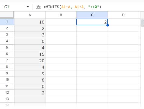
The following formula will return the minimum value excluding zeros in column A in Google Sheets:
=MINIFS(A1:A, A1:A, "<>0")
This follows the syntax:
MINIFS(range, criteria_range1, criterion1, [criteria_range2, …], [criterion2, …])Where:
range: A1:Acriteria_range1: A1:Acriterion1: “<>0”
The MINIFS function returns the minimum value by filtering the criteria range based on the provided condition, which is “<>0”.
FILTER and MIN Solution
Here, we use the FILTER function to filter the range and then apply MIN to that filtered range:
=MIN(FILTER(A1:A, A1:A<>0))It follows the FILTER syntax:
FILTER(range, condition1, [condition2, …])Where:
range: A1:Acondition: A1:A<>0
From the above two formulas, I recommend using MINIFS because it can return the min value excluding zeros in a 2D array as well.
MIN Excluding Zeros in a 2D Array in Google Sheets
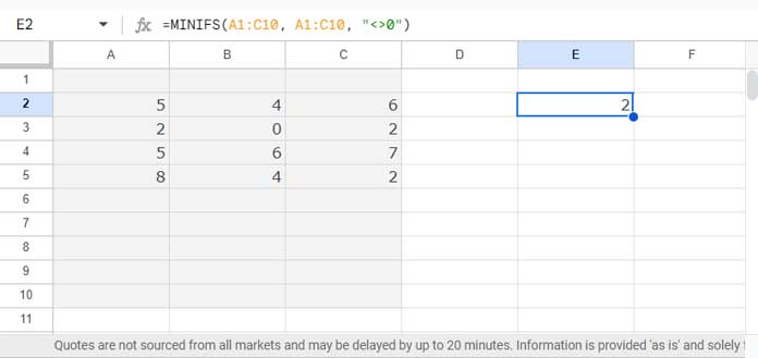
Assume you want to extract the minimum value excluding zeros in A1:C10, a 2D array.
The MINIFS formula will work without any issues:
=MINIFS(A1:C10, A1:C10, "<>0")
However, the FILTER and MIN combination won’t work directly because the ‘condition’ part in the FILTER function should be one-dimensional.
To handle this, use the TOCOL function to convert the 2D array to a one-dimensional array. Here is the combination:
=MIN(FILTER(TOCOL(A1:C10), TOCOL(A1:C10)<>0))Why Does the MINIFS Formula Return 0?
When the range to find the min excluding zero is blank, MINIFS will return 0, and the FILTER+MIN combination will return a #N/A error.
How do I return an empty cell instead?
If you use the FILTER and MIN combination, simply wrap it with the IFNA function:
Example:
=IFNA(MIN(FILTER(A1:A, A1:A<>0)))But if you use MINIFS, it’s not as straightforward. You should use an IF logical test:
=LET(test, MINIFS(A1:A, A1:A, "<>0"), IF(test<>0,test,))Resources
- Find Minimum Value and Return Value From Another Column
- How to Use MIN in Array in Google Sheets for Expanded Results
- Find Min, Max in a Matrix and Return a Value from the Same Row in Sheets
- Hyperlink Max and Min Values in Column or Row in Google Sheets
- Row-Wise MIN Using DMIN in Google Sheets
- How to Retrieve Column Header of Min Value in Google Sheets
- Get Min Date Ignoring Blanks in Each Row in Google Sheets
- Filter Min or Max Value in Each Group in Google Sheets
- Find the Running Minimum Value in Google Sheets


One other thing I left out. Another thing I need to do is, once the array finds the lowest value excluding zero, I need it to return the name of the lowest value. Same for the second, third, and lowest overall.
Thank you,
Nuria
Hi, Nuria Anderson,
I think I can help you here.
We can use Query or ArrayConstrain+Sort. It depends on your data.
Can you prepare and share a sample sheet? So that I can write the formula and share the steps on the sheet.
You can leave the URL via “Reply” to this comment (I won’t publish it).
I found your answers to be very helpful when other places were of no help whatsoever. I need an additional step, however.
My data is in every other column (think the description in one and pricing on the other, so the numbers are in every other column). I need to find the first lowest excluding zero, which I have done with the Query.
Thank you for that, by the way!
Now in the same array, I need to find the second-lowest, third lowest, and overall lowest number.
How do I do that?
I appreciate your insight on this.
Thanks again!
Hi, Nuria Anderson,
Instead of
min(query);Use
small(query,1)for the min value,small(query,2)for the second lowest value and so on.