


This tutorial elaborates on the use of Countifs with Isbetween in Google Sheets. In the course, you may learn to use other matching criteria with them.
For example, assume you want to find how many times you filled fuel in your vehicle during a given period.
In Countifs, you can use Isbetween to match the start and end dates (given period) in a date column, and “fuel” will be the other matching criteria in a category column.
You may find this combo worthwhile if you often get formula mistakes because of the erroneous use of comparison operators.
Comparison operators in Countifs need to enter in double quotation marks. This is often overlooked as other functions like Filter do not require it.
Instead of comparison operators >, >=, <, <=, you can use the Isbetween function with Countif or Coutifs in Google Sheets.
Ideally, you can use Countifs with Isbetween to count values that fall within two dates or numbers and one or more corresponding/matching criteria.
Countifs with Isbetween in Google Sheets: How to
Countifs Function Syntax: COUNTIFS(criteria_range1, criterion1, [criteria_range2, …], [criterion2, …])
The structure of our familiar Countifs formula radically changes when we change the comparison operators to Isbetween.
We use comparison operators within the criterion part whereas the alternative Isbetween with the criteria_range part.
Then what about the criterion in this (Isbetween) case?
We should change it to Boolean TRUE. Below you can find two formula examples of Countifs with Isbetween use.
Example 1: Countifs Between Two Dates
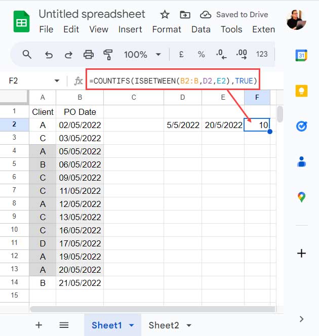
In the following example, column A displays the client names and column B displays the PO dates.
How do we use the Countifs function to find the number of POs between a start date (D2) and an end date (E2)?
Formula:
=COUNTIFS(ISBETWEEN(B2:B,D2,E2),TRUE)Where;
criteria_range1: ISBETWEEN(B2:B,D2,E2)
criterion1: TRUE
In the Countifs and Isbetween combo above, would you like to know the role of the latter function?
Then please check the below screenshot.
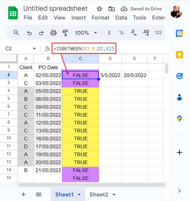
Syntax of Isbetween: ISBETWEEN(value_to_compare, lower_value, upper_value, [lower_value_is_inclusive], [upper_value_is_inclusive])
The Isbetween function tests whether the PO Date (value_to_compare) falls within the start date (lower_value) and end date (upper_value) and returns TRUE or FALSE.
The Countifs returns the count of Boolean TRUE values.
In my formula, lower_value and upper_value are inclusive. If you want to exclude, specify FALSE as below.
=COUNTIFS(ISBETWEEN(B2:B,D2,E2,FALSE,FALSE),TRUE)In the next example, we will see how to Countifs between two dates and matching criteria from another column.
Example 2: Countifs Between Two Dates and Matching Criteria
The data range is the same here, i.e., the Client and PO dates in columns A and B.
The cell references for the criteria are the start date in D2, the end date in E2, and the client name “C” in F2.
In this Countifs with Isbetween formula, we want to find the number of POs received from client “C” from 05/05/2022 to 20/05/2022.
=COUNTIFS(ISBETWEEN(B2:B,D2,E2),TRUE,A2:A,"A")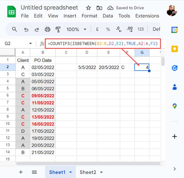
What about counting the purchase orders received between 05/05/2022 and 20/05/2022 from clients “A” and “D”?
Aside from the three criteria above, suppose we have the client name “D” in cell F3.
Then we can use the following formula.
=ARRAYFORMULA(SUM(COUNTIFS(ISBETWEEN(B2:B,D2,E2),TRUE,A2:A,{F2,F3})))Placed those text criterion references as an array using Curly Brackets and additionally used Sum and ArrayFormula functions.
You can find a similar usage here: OR in Multiple Columns in COUNTIFS in Google Sheets.
That’s all about Countifs between two dates and matching multiple criteria in Google Sheets.
Countifs with Isbetween and Multiple Start and End Dates
You can follow two methods when you want to test multiple sets of start and end dates in Countifs with Isbetween use.
One is a drag-down formula, and the other is a Lambda formula.
You already have the drag-down formula above. In that, you need to replace B2:B with $B$2:$B and A2:A with $A$2:$A before dragging down. That’s it.
What about an array (spill down) formula?
When you want to test multiple sets of start and end dates, you can take the help of the Map Lambda function.
That’s the easiest way to spill a Countifs with Isbetween down.
Example:
=MAP(D2:D4,E2:E4,LAMBDA(start,end,COUNTIFS(ISBETWEEN(B2:B,start,end),TRUE)))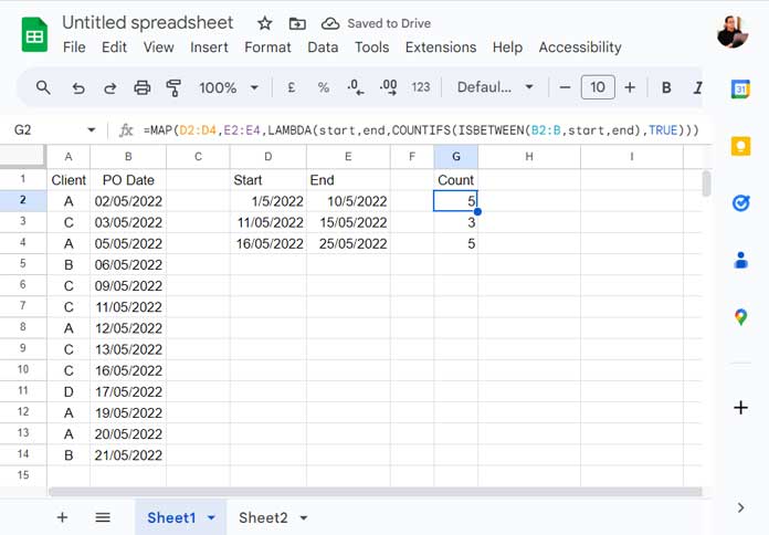
What about Countifs between two dates and matching criteria and spill down?
Fill F2:F4 with the client name “A.”
Then use this Map formula.
=MAP(D2:D4,E2:E4,F2:F4,LAMBDA(start,end,client,COUNTIFS(ISBETWEEN(B2:B,start,end),TRUE,A2:A,client)))Note:- Avoid any blank cell in the criteria range.
Conclusion
Most of you may not find problems using the above Countifs with Isbetween formulas in different ranges in your worksheets.
In case of any issues, I suggest you first use the above formulas in the same data ranges in my example.
Then you can insert columns or rows to move the ranges. The formula will adjust accordingly.
If you have any other issues, please post in the comments. I’ll get back to you ASAP.
Here are some related resources that you may find useful.
- COUNTIFS in a Time Range in Google Sheets [Date and Time Column].
- COUNTIF to Count by Month in a Date Range in Google Sheets.
- Count Unique Dates in a Date Range – 5 Formula Options in Google Sheets.
- Count Values Between Two Dates in Google Sheets.