Using COUNTIFS with time ranges in Google Sheets involves applying this function to a time column or a timestamp column. Each requires a slightly different technique.
In essence, a time range here refers to specific intervals, such as one-hour or two-hour segments. For instance, you might want to count all activities or tickets recorded between 8:00:00 AM and 10:00:00 AM. The column being evaluated could contain either time values or timestamps (date and time).
Using COUNTIFS with Time Ranges in a Time Column
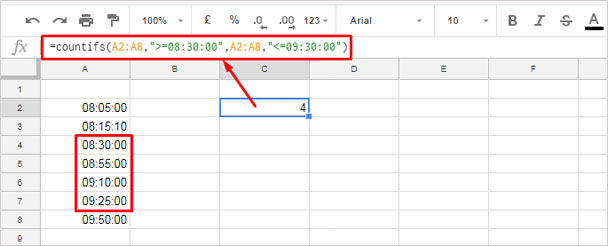
Here’s an example of how to use COUNTIFS with a time range when the column contains only time values in Google Sheets.
The following formula counts entries in column A, range A2:A8, that fall within the time range from 08:30:00 to 09:30:00, inclusive:
=COUNTIFS(A2:A8, ">=08:30:00", A2:A8, "<=09:30:00")
Alternatively, you can input the criteria into cells (e.g., E2 for 08:30:00 and F2 for 09:30:00) and refer to those cells in the formula:
=COUNTIFS(A2:A8, ">="&E2, A2:A8, "<="&F2)Counting time by duration is straightforward when working with pure time values. However, things become more complex if column A contains timestamps (dates and times) rather than just time values.
Using COUNTIFS with Time Ranges in a Date-Time Column
The solution depends on whether you want to include the date in the criteria or not. If you don’t need the date, you’ll need to extract the time component from the timestamp and use it in the formula. Let’s explore both scenarios:
Using Date and Time Criteria with COUNTIFS
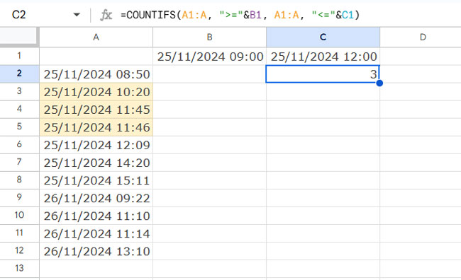
Suppose you’ve recorded material delivery times (timestamps) in column A and want to count the number of trucks that arrived between 09:00 AM and 12:00 PM on a specific date.
You can use the following COUNTIFS formula:
=COUNTIFS(A1:A, ">=2024-11-25 09:00:00", A1:A, "<=2024-11-25 12:00:00")Here, the date is specified in ISO 8601 format (YYYY-MM-DD) to avoid confusion caused by regional date formats, such as DD/MM/YYYY or MM/DD/YYYY.
Alternatively, you can input the start and end datetime values into two cells (e.g., B1 and C1) and use them in the formula:
=COUNTIFS(A1:A, ">="&B1, A1:A, "<="&C1)
Using Time Criteria with COUNTIFS
What if you want to count entries within a specific time range, regardless of the date? For instance, you might want to find how many trucks arrived between 09:00 AM and 12:00 PM on any day.
Here, you need to extract the time component from the timestamp column. Two approaches can help:
- Using SPLIT and CHOOSECOLS:
=ArrayFormula(CHOOSECOLS(SPLIT(A:A, " "), 2))This splits the timestamp into date and time and selects the time component. - Using MOD:
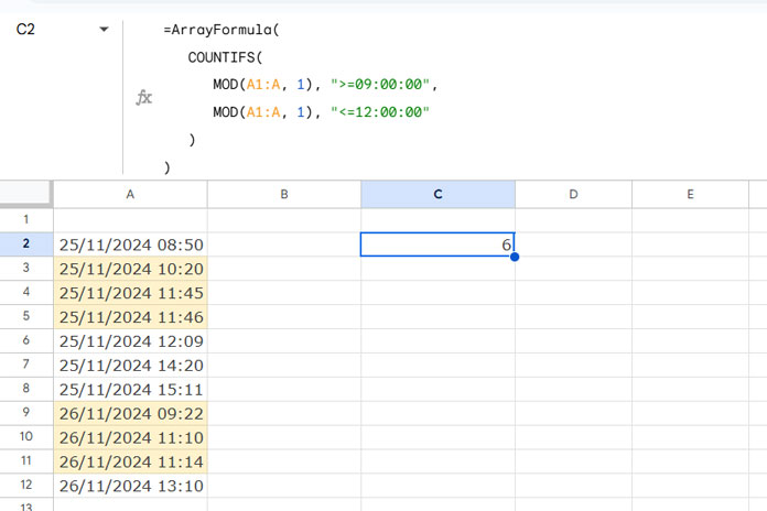
=ArrayFormula(MOD(A1:A, 1))The MOD function extracts the time component by calculating the remainder when the datetime is divided by 1 (dates are integers, and times are fractional).
You can use either method in the range part of your COUNTIFS formula:
=ArrayFormula(
   COUNTIFS(
      CHOOSECOLS(SPLIT(A:A, " "), 2), ">=09:00:00",
      CHOOSECOLS(SPLIT(A:A, " "), 2), "<=12:00:00"
   )
)
or
=ArrayFormula(
   COUNTIFS(
      MOD(A1:A, 1), ">=09:00:00",
      MOD(A1:A, 1), "<=12:00:00"
   )
)
Conclusion
We’ve explored how to use COUNTIFS with time ranges in both time and datetime columns. In all examples, we used comparison operators (>= and <=) to make the criteria inclusive. If you prefer exclusive criteria, replace them with > and <.
For further flexibility, consider using the ISBETWEEN function to simplify the formula. You can find more examples of COUNTIFS usage with ISBETWEEN in the resource section below.
If you’d like to explore other ways to count events by timeslot — including using FILTER, SUMPRODUCT, QUERY, and Pivot Tables — check out our full guide: Count Events by Timeslot in Google Sheets — 4 Easy Methods.
Resources
- COUNTIFS with Multiple Criteria in the Same Range in Google Sheets
- COUNTIFS with ‘Not Equal To’ in Infinite Ranges in Google Sheets
- Using ‘Not Blank’ as a Condition in COUNTIFS in Google Sheets
- COUNTIF | COUNTIFS Excluding Hidden Rows in Google Sheets
- How to Use COUNTIF or COUNTIFS in Merged Cells in Google Sheets
- Handling Varying Array Sizes in COUNTIFS in Google Sheets
- OR Logic in Multiple Columns with COUNTIFS in Google Sheets
- OR Logic in COUNTIFS Across Either Column in Google Sheets
- COUNTIFS with ISBETWEEN in Google Sheets
- Counting XLOOKUP Results with COUNTIFS in Excel and Google Sheets


Hi, how about this one?
In Column A:
ROW 2 (May 1, 2024)
ROW 4:
01/05/2024 15:10
01/05/2024 15:04
01/05/2024 15:10
01/05/2024 16:16
02/05/2024 14:55
02/05/2024 15:49
02/05/2024 15:01
03/05/2024 14:55
03/05/2024 14:49
I want to count the data with the date in Row 2 from 15:00 to 16:59. Thanks for your answer.
You can try this combination of COUNTIF and ISBETWEEN:
=COUNTIF(ISBETWEEN(A4:J4, A2+TIME(15, 0, 0), A2+TIME(16, 59, 0)), TRUE)Prashanth,
I have a tricky one for you. I have data that is constantly auto-populating. The data is; package number, Status (Enroute, Arrived, Pending, Accepted), and date with time. I want to use a countif formula to know how many different statuses I have but only count the most up-to-date information.
Example:
I might have 10 entries for package Number 1. They are all time-stamped with varying statuses, but I only want to count package number 1 status once and based on its latest time stamp. I then want to add that single count for that package number with all the other most up-to-date package number counts.
Basically, I want to know how many Enroute statues I have but only based on the most recent submissions. Can google sheets do this? Is there a formula for this?
As always thank you so much for your help and all that you do. I very much appreciate it.
Hi, Monk,
This formula might help you to find the most recent “Enroute” statuses.
=sortn(sort(filter(indirect("A2:C"),indirect("B2:B")="Enroute"),3,0,1,1),9^9,2,1,1)
It would return results in two columns and multiple rows. So make two columns empty and insert the formula in the first cell of the first column.
To get the count, you can use this formula.
=counta(index(sortn(sort(filter(indirect("A2:C"),indirect("B2:B")="Enroute"),3,0,1,1),9^9,2,1,1),0,1))
If that doesn’t help, please prepare and share an example Sheet (URL) via the comment below.
Hi, can someone please help me to correct my function?
Count the number of cells with Date “Today” and Time “between 06:00 and 14:30″
=countifs('A:A">=Today() 06:00:00", 'A:A"<=Today() 14:30:00")Thanks
Hi, Alaa,
Here is the correct way to add time to today’s date.
=today()+TIME(hour, minute, second)So the formula will be;
=countifs(A:A,">="&Today()+time(6,0,0), A:A,"<="&Today()+time(14,30,0))Hi,
Thank you for this post. It has been the only formula that would work for what I wanted to do.
I do seem to have a problem with Formula 4 picking up midnight in the time range…”00:00″.
My formula is below:
=ArrayFormula(COUNTIFS(value(replace(AM3:AM50,1,11,)),”>=23:01″,VALUE(REPLACE(AM3:AM50,1,11,)),”<=00:00"))
AM3:AM50 contains this in one of its cells: 23 Jan 2020 00:00
However, this cell is not being included in the count.
Thank you so much.
Hi, Angie,
I guess the first DateTime is 23/01/2020 23:01 and the second DateTime is 23/01/2020 00:00. That means the second date is less than the first date as the time 00:00 means 12:00 am. So the formula won’t include the same in the count.
For including midnight time falls on the same day, try the second criterion as 23:59 instead of 00:00.
Best,