QUERY and Pivot Table are two options in Google Sheets for combining and summing duplicate or similar rows. However, you can also use a unique combination formula with UNIQUE and SUMIF. In this tutorial, I’ll detail all three options so you can choose the one that best suits your needs.
For clarity, I’m using a very basic data set so that you can easily follow the steps.
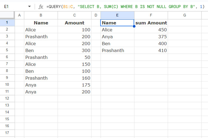
In the first example, I’ll use a two-column data set: names in the first column (B1:B) and amounts in the second column (C1:C).
| Name | Amount |
| Alice | 100 |
| Prashanth | 200 |
| Alice | 200 |
| Ben | 300 |
| Prashanth | 50 |
| Alice | 150 |
| Ben | 100 |
| Prashanth | 160 |
| Anya | 175 |
| Anya | 200 |
In the final part of this tutorial, you’ll learn how to apply these techniques to multiple columns for similar calculations.
Combine Similar Rows and Sum Values: Single-Column Grouping
QUERY is one of the quintessential functions for data manipulation in Google Sheets. So let’s start with that.
Option 1: QUERY
Even if you’re unfamiliar with the QUERY function, you can follow my formula to gain the basic skills needed to combine similar rows and sum values in Google Sheets.
Formula:
=QUERY(B1:C11, "SELECT B, SUM(C) GROUP BY B", 1)This formula selects the names in column B and calculates the total in column C by grouping the names in column B.
If you want to include an unlimited number of rows in the QUERY to account for future values, modify the formula as follows:
=QUERY(B1:C, "SELECT B, SUM(C) WHERE B IS NOT NULL GROUP BY B", 1)Option 2: SUMIF and UNIQUE
This method involves two steps:
- First, enter the following UNIQUE formula in cell E2 to get the unique categories (names) in column B:
=UNIQUE(B2:B)- Then, in cell F2, enter the following SUMIF array formula to sum the values in the range C2:C that match the unique categories in B2:B:
=ArrayFormula(SUMIF(B2:B, E2:E, C2:C))This formula may leave trailing zeros where E2:E is empty. If you want to avoid that, use this formula instead:
=ArrayFormula(IF(E2:E="",,SUMIF(B2:B, E2:E, C2:C)))That’s how we combine similar rows and sum values using the SUMIF and UNIQUE combination. Now, let’s move on to the Pivot Table.
Option 3: Pivot Table
If you’re not comfortable with formulas, a Pivot Table is your best option.
A Pivot Table is a built-in tool for summarizing and analyzing data in popular spreadsheet applications. You can use it to combine and sum similar rows in Google Sheets as follows:
- Select the range B1:C.
- Click Insert > Pivot Table.
- Click Create.
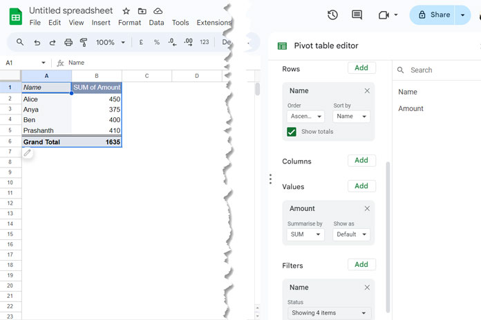
- This will open a new sheet with the Pivot Table layout and a sidebar panel on the right-hand side.
- In the sidebar, drag and drop the “Name” field (the group column header) under “Rows.”
- Then, drag and drop the “Amount” field (the sum column header) under “Values.”
- Drag and drop the “Name” field under “Filter.”
- In the Filter field, click the “Show all items” drop-down and uncheck “(Blanks).”
This is the non-formula approach to combining similar rows and summing values.
Combine Duplicates in Rows and Sum Values (Multiple Columns)
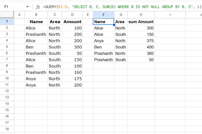
This time we have a three-column data set where column B contains names, column C contains areas, and column D contains amounts.
For this data set, you can use either QUERY or a Pivot Table.
I don’t recommend the SUMIF and UNIQUE combination as it won’t automatically expand the results. To handle this, you might consider combining names and areas or using the MAP LAMBDA function, which can be complex for beginners.
Here is the QUERY formula to combine duplicates in rows and sum values based on the category and subcategory columns:
=QUERY(B1:D, "SELECT B, C, SUM(D) WHERE B IS NOT NULL GROUP BY B, C", 1)If you prefer using a Pivot Table, the only change compared to the two-column data set is:
- Drag and drop the Area field under “Rows,” below the Name field.


This query formula opened up a whole new world to me. Thanks!
Hi, I’m working on similar to it.
I need to combine a duplicate row and sum the values of 2 columns differently.
After getting that, I need to combine my filter function with the query function.
Filter Function:
=filter(C5:E,A5:A=B1)[this is for the dropdown category]Hi, ching,
I’m not clear. Please feel free to share an example (sheet).
Hello,
I am doing something similar, but I need to separate the data by date. I cannot seem to get the formula right. Can you assist?
Hi, Janira Iglesias,
Here is an example.
Data in Columns:
A – Dates
B – Item Description
C – Quantity.
The formula in D1:
=query(A1:C,"Select A,B,sum(C) where A is not null group by A,B")Please try it first. If that doesn’t help, make a sample and share that Sheet’s address/URL via the comment below.
Hi Prashanth,
hope you are well. First of all thanks so much for sharing your knowledge with the world. Very highly appreciated.
I would have one question sum values part. I used your Merge/Combine rows solutions and it’s working fine for my use case. Except for one part.
I’m using it for consolidation Orders from an e-commerce shop so I get one row per Order showing all different order positions and items that are in one basket/order.
So origin Data shows two rows when two items are ordered. In one column it says “order position number” ..and because it’s two items its two rows with “order position number” #1 and the next row #2.
I would like to not sum up but only show in the final table “order positions: #2” (as there are two items). Summing up would show #3.
So is there a way to either only take the second value = #2 or identify the highest value? (it could also be somebody orders 5 times the same item, then I would have 1 row for the order showing order positions =5)
Hi, Felix,
Please feel free to share a mockup (sample) sheet. I think I can help you write the required formula.
Hello, are you still taking inquiries? I am trying to consolidate two sets of information that have repeating values (as shown in your video) but I would like a different result. Are you still monitoring this?
Thanks!
Hi, Louie N,
Nope! But I’ll try to help you in my leisure if you can share with me a sample of what you are working on. Use the ‘Reply’ below to share yours sheet. The link won’t be published here to protect your privacy.
NB: Just a sample in 5-10 rows and a few columns.
Need help! The array formula calculates all blank cells too. How to get rid off it?
The below formula is as per the sample data and the formula used in the example in my tutorial.
=ArrayFormula(if(len(G4:G),sumif(B3:B&C3:C,G4:G&H4:H,D3:D),))In your case, it might be
len(K2:K)Best,
Hey Prashanth,
I’m still having issues doing this. Since I can’t post a screenshot, I will try to explain it here.
Column C has Multiple Values (Will Continue to grow with different Values)
Column D has Multiple Values (Will Continue to grow with different Values)
Column E is what I need the SUM for and is numeric
Thank you in advance,
Adam B. Yuro
Hi, Adam,
You can try this Query. In this row#1 is considered as the header row.
=query(C1:E,"Select C,D, sum(E) where C is not null group by C,D",1)If there is no header, then the Query formula would be like this.
=query(C1:E,"Select C,D, sum(E) where C is not null group by C,D",0)Both of these formulas won’t work if you are from EU countries. Then use the Query as below.
=query(C1:E;"Select C,D, sum(E) where C is not null group by C,D";1)If not helpful? Then try to share your Sheets’ link (no personal/confidential data)
Best,
This is great and thank you! Is there a way to not make the resulting data a new set of columns, but rather rearrange and modify the original data to show the sums?
Hi, Mark J.,
Please share the screenshot of your example data and the expected result.