The CODE function in Google Sheets returns the Unicode code point value of a character. This function provides a numeric output. If you are looking for a function to return characters like “©,” “µ,” “¾,” etc., consider using the CHAR function.

If you use a text string instead of a single character in the CODE function, it will return the value of the first character, and other characters in the string will not be considered.

In Google Docs Spreadsheet, I typically use the CODE function to determine the value of the output from the CHAR function.

I recently employed these functions in a tutorial to create complex passwords based on provided names and dates of birth.

Therefore, you should understand what the CODE function is and how it differs from the CHAR function in Google Sheets.

As a side note, you can use the UNICODE function instead of the CODE function in Google Sheets. Why are there two functions?

The presence of both functions is due to compatibility with Excel, which includes both CODE and UNICODE functions. The CODE function was introduced in earlier versions of Excel, which initially supported the ANSI/Macintosh character set. In Google Sheets, the CODE function has been expanded to encompass Unicode characters, providing broader character support.

Syntax and Argument

Here is the syntax of the CODE Function in Google Sheets:

CODE(string)

string: Required. The string for which you want the code of the first character.

Decoding Character Conversions: Comparing the CODE and CHAR Functions in Google Sheets

Let’s explore the relationship between the CODE and CHAR functions with a few examples below.

Example #1:

The following CODE formula returns the Unicode value of the Omega character:

=CODE("Ω")  // returns 937

Whereas the following CHAR formula returns the Omega character:

=CHAR(937)  // returns "Ω"

Example #2:

The following formula returns the numerical Unicode code point of the first character, which is “A,” in the word “APPLE”:

=CODE("APPLE")  // returns 65

Therefore, the following CODE formula would also return the value 65 for the character “A”:

=CODE("A")  // returns 65

Now, let’s consider the CHAR formula:

The formula =CHAR(65) would return the character “A”.

I hope this helps you understand how to use the CODE function in Google Sheets.

Note: The Unicode values of the capital letters (English alphabets) A to Z range from 65 to 90, and the small letters range from 97 to 122.

Practical Use of the CODE Function in Google Sheets:

You can employ the CODE function to convert a case-insensitive formula into a case-sensitive one in a clever way. To see this in action, take a look at my case-sensitive VLOOKUP formula where I’ve utilized the CODE function.

Unicode Characters and Map Values in Google Sheets

You can refer to this wiki page to find Unicode characters and their code values. Here are some of the most useful ones (screenshot).

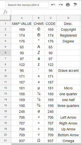
In this example, I’ve used the formula =CHAR(A2) in cell B2 and dragged it down. In cell C2, there is a CODE formula =CODE(B2) that is also dragged down to fill the cells.

I personally don’t find much use for this function, but it may have different applications for you. For me, the CHAR function is quite useful in Google Sheets.

Feel free to explore some of my tutorials that demonstrate how to maximize the benefits of the CHAR function in Google Sheets.

Related:

1. How to Get Subscript and Superscript Numbers in Google Spreadsheets.
2. 5-Star Rating in Google Sheets Including Half Stars.
3. How to Create a Percentage Progress Bar in Google Sheets.
4. Insert Special Characters Without Add-on in Google Sheets.
5. Inserting Bullet Points in Google Sheets.