You can use my formula to easily generate a list of passwords in Google Sheets. To create passwords, I am using usernames and their dates of birth. The passwords will be strong, as they’ll be a mix of alphanumerics and, optionally, special characters. Also, you can customize the password so that not all readers of this tutorial end up creating the same passwords if they use the same username and date of birth.
You can use my method to generate strong passwords in Google Sheets for your students or for employees in your organization to access their office-related accounts.
However, I do not recommend using this formula to create passwords for securing important online accounts like banking, websites, domains, hosting, insurance accounts, etc. That doesn’t mean the passwords generated with Google Sheets are weak—it’s just always better to use highly specialized tools for sensitive accounts.
We’ll create the passwords step-by-step so that each of you can add your personal flavor and make them unique to you.
Steps to Generate a List of Strong Passwords in Google Sheets
1. Preparing the Names and Dates of Birth
As I mentioned above, we’ll generate passwords in Google Sheets using usernames and their DOBs.
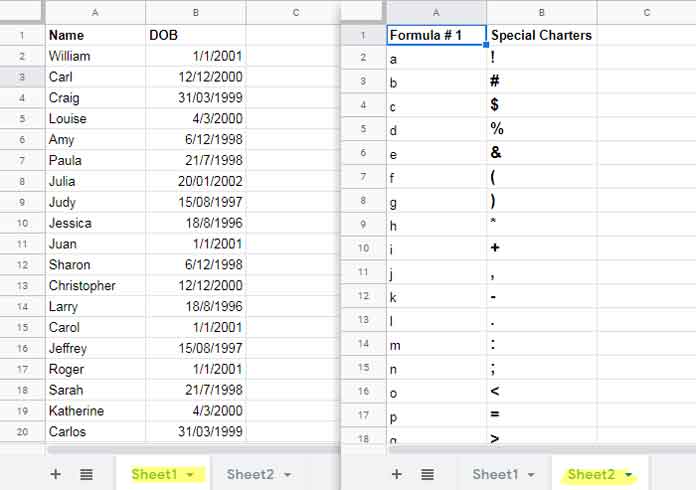
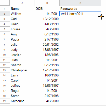
In “Sheet1,” enter usernames (student or employee names) in column A and their dates of birth in column B. Do not include spaces in the usernames. For example, “Prashanth KV” must be entered as “PrashanthKV”.
2. Preparing the Lookup Table to Assign Special Characters
If your service or platform accepts special characters in passwords, you can specify them here. If not, you can use any digits. Let me explain.
In “Sheet2,” cell A2, enter the following formula to generate the alphabet a to z:
=ArrayFormula(CHAR(SEQUENCE(26, 1, 97)))(You can find a detailed explanation here: How to Autofill Alphabets in Google Sheets.)
In column B (next to the alphabet list), manually enter the special characters you want to include in your passwords. Here’s a sample list:
- Punctuation marks:
! @ # $ % ^ & * ( ) _ - + = - Brackets/braces:
{ } [ ] ( ) - Math/logic symbols:
< > = - Others:
~ | \ : ; " ' , . ? /
There are 26 letters in column A, so you should have 26 corresponding symbols in column B.
Tip: You can either repeat symbols or use unique ones.
If your platform doesn't accept symbols, you can simply use numbers 0 to 9 (in any order) in B2:B27.
This lookup table ensures that every user generates a strong and unique password in Google Sheets based on their custom symbols or numbers.
3. Randomly Capitalize Letters in a Name to Generate a Basic Password
Mixing uppercase and lowercase letters makes passwords stronger. Since we aim to generate a list of strong passwords in Google Sheets, we can’t skip this step.
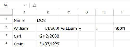
In cell C2 of “Sheet1,” enter this formula:
=JOIN("", LET(letters, SPLIT(REGEXREPLACE(LOWER(A2), "(.{1})", "$1,"), ","), ARRAYFORMULA(IF(ISEVEN(CODE(letters)), CHAR(CODE(letters)-32), letters))))You’re free to replace ISEVEN with ISODD if you want a different randomization.
Quick Explanation:
i) Splitting Each Character in the Name
The REGEXREPLACE function adds commas between letters, and SPLIT separates them into columns. LOWER ensures everything starts lowercase.
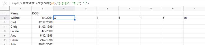
ii) Using the CODE Function to Capitalize Random Letters
The CODE function gets the ASCII code of each character. If it’s an even code, subtract 32 to turn it into an uppercase letter.
iii) Joining the Characters
Finally, JOIN puts the letters back together.
For example, “William” might turn into:
wiLLiam
4. Add Special Characters Randomly to the Generated Password
Now let’s add special characters using XLOOKUP.
First, we’ll pick a special character based on the second character of the username:
In cell D2:
=XLOOKUP(MID(A2, 2, 1), Sheet2!$A$2:$A$27, Sheet2!$B$2:$B$27)(Here, 2 in MID(A2, 2, 1) controls which character is used.)
Next, we’ll pick another special character based on the last character:
In cell E2:
=XLOOKUP(RIGHT(A2, 1), Sheet2!$A$2:$A$27, Sheet2!$B$2:$B$27)Tip: You can useLEFTinstead ofRIGHTif you want to vary the formula.
5. Additional Characters from Date of Birth to Add to the Password
Let’s spice it up by pulling characters from the user’s date of birth:
In cell F2:
=RIGHT(TEXT(B2,"mmm"), 1)&MID(TEXT(B2, "yyyy"), 2, 3)&DAY(B2)This formula returns:
- The last character of the abbreviated month name,
- The middle three digits of the year,
- The day of birth.
You can customize this further by adjusting which parts of the DOB you include.
6. Generating a List of Strong Passwords in Google Sheets
Now, let’s combine everything into one formula.
In cell G2:
=D2&C2&E2&F2Or, if you prefer a single formula (without using intermediate columns), here it is:
=XLOOKUP(MID(A2,2,1),Sheet2!$A$2:$A$27,Sheet2!$B$2:$B$27)&JOIN("", LET(letters, SPLIT(REGEXREPLACE(LOWER(A2),"(.{1})", "$1,"), ","), ARRAYFORMULA(IF(ISEVEN(CODE(letters)), CHAR(CODE(letters)-32), letters))))&XLOOKUP(RIGHT(A2, 1), Sheet2!$A$2:$A$27, Sheet2!$B$2:$B$27)&RIGHT(TEXT(B2,"mmm"), 1)&MID(TEXT(B2, "yyyy"), 2, 3)&DAY(B2)Enter this final formula in cell C2 and copy it down as far as needed.
FAQs – Generating a Strong List of Passwords in Google Sheets
Q: Does this formula support special characters?
A: Yes, you can customize it to include any special characters you like.
Q: Can I generate passwords with only alphanumerics?
A: Absolutely! Just use numbers or letters instead of special characters in your lookup table.
Q: Are the passwords strong enough?
A: They are strong for general usage (like student/employee accounts), but for critical online services, use a professional password manager.
Q: Is the password generator customizable?
A: Yes, you can tweak capitalization rules, symbols, lookup positions, and DOB patterns to fit your needs.


