If you’re looking for a flexible array formula to join columns in Google Sheets, you’re in the right place! I have two of the best solutions to share. We can join columns using a simple Query formula.
Typically, we rely on the JOIN, TEXTJOIN, CONCATENATE, CONCAT functions, and the ampersand to combine values. However, none of these fully support arrays in the way we need.
The first three are not suitable for combining entire columns, as they return a single value instead of working row by row.
The CONCAT function can combine columns but lacks flexibility, as it only supports two arrays and doesn’t allow for a delimiter.
The ampersand is a better option, though it’s not dynamic. You must specify each column individually.
But I have a simple and elegant solution using a Query that works with both physical and virtual columns.
Update: We can now use JOIN and TEXTJOIN functions with a supporting Lambda helper function to achieve the desired results.
Joining Columns Using JOIN, TEXTJOIN, and CONCATENATE Functions
We’ll start with drag-down formulas to combine columns.
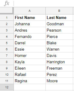
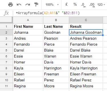
We’ll use a sample data set that contains first names in A2:A11 and last names in B2:B11, and we’ll combine them in C2:C11.

Insert any of the following formulas in cell C2 and drag it down as far as needed:
=JOIN(" ", A2:B2)
=CONCATENATE(A2, " ", B2)
=TEXTJOIN(" ", TRUE, A2:B2)
In all three formulas above, the space is the delimiter that separates the first and last names.
The TEXTJOIN function has an added advantage: it won’t add the delimiter if you forget to enter the first or last name. This ensures that the output looks clean, especially when the delimiter is not a space but a comma, pipe, or another character.
We can’t use the CONCAT function, as it doesn’t have the option to place a delimiter—it simply combines two columns.
All of the above are non-array formulas for joining columns. However, we can convert them to flexible array formulas using the BYROW and LAMBDA functions, which we’ll explore later.
Note: If you have three columns, the formulas will look as follows:
=JOIN(" ", A2:C2)
=CONCATENATE(A2, " ", B2, " ", C2)
=TEXTJOIN(" ", TRUE, A2:C2)
Array Formula Approach Using Ampersand (Non-Flexible)
I might recommend using the ampersand if you ask me which is the easiest array formula method to join columns in Google Sheets.
=ArrayFormula(A2:A11&" "&B2:B11)
There is one drawback:
- You need to specify the columns individually, not as a range, making it non-flexible.
If you have one more column, the formula would look something like this:
=ArrayFormula(A2:A11&" "&B2:B11&" "&C2:C11)Flexible Array Formula to Join Columns in Google Sheets – QUERY
First, let’s look at the formula:
=TRANSPOSE(QUERY(TRANSPOSE(A2:B11), , COLUMNS(A2:B11)))This is called a flexible array formula because it uses a range instead of specifying columns individually to join columns.
Anatomy of the Formula:
Here’s the syntax: QUERY(data, query, [headers])
If you use the QUERY function without a query parameter, it will return the data as is.
In our Query, the transposed range A2:B11 is the data:
=QUERY(TRANSPOSE(A2:B11))
We have transposed two columns into two rows. We need to tell the Query that these two rows are headers:
=QUERY(TRANSPOSE(A2:B11), , 2)Result:

Instead of hardcoding the number 2, we use the COLUMNS function to dynamically return the number of columns in the data range A2:B11 (which corresponds to the number of rows in the transposed data range A2:B11).
That’s what I did—then I transposed the data once again.
Flexible Array Formula for Joining Columns in Google Sheets Using BYROW
Using BYROW, one of the Lambda helper functions, we can enhance the results of the text functions mentioned earlier in this tutorial. I am choosing TEXTJOIN because it can omit blank cells.
Here is the next flexible array formula to join columns in Google Sheets:
=BYROW(A2:B11, LAMBDA(r, TEXTJOIN(" ", TRUE, r)))The unnamed LAMBDA function joins the first and last names using TEXTJOIN, and BYROW iterates over each row in the array, making it a dynamic array formula.
Which Dynamic Formula Is Right for Me?
I suggest using QUERY if you have very large data and want a space as the column separator. If you need to control the delimiter and achieve a clean output, BYROW is the best option.
However, BYROW is a LAMBDA helper function that might encounter performance issues with very large data sets.
Resources
- How to Remove Extra Delimiter in Google Sheets – Join Columns
- How to Left Join Two Tables in Google Sheets
- How to Right Join Two Tables in Google Sheets
- How to Inner Join Two Tables in Google Sheets
- How to Full Join Two Tables in Google Sheets
- Master Joins in Google Sheets (Left, Right, Inner, & Full) – Duplicate IDs Solved
- Anti-Join in Google Sheets: Find Unmatched Records Easily
- Google Sheets: Combine Tables with Unequal Columns in QUERY
- Query to Combine Columns and Adding Separators in Google Sheets


Is there a way to insert a unique delimiter between the penultimate and last values for each row?
What I am trying to do is add an “and” before the last value in a comma-separated list.
Hi, Misha,
Assume the comma-separated texts are in the A2:A range.
Then try this formula in B2 (first empty column B).
=ArrayFormula(regexreplace(A2:A, "(.*),", "$1, and "))Related: Regex to Replace the Last Occurrence of a Character in Google Sheets.
Amazing… thanks for this…
It exactly worked as advertised, thank you very much.
Great solution! I often use this to manage CSV files. But how to join only unique columns? Thank you.
This is what I needed! In the last formula you used, how can I put a separator between the combined values?
Hi, Robert Petitto,
Here is the Query formula to combine columns and put a separator between the combined values.
=ArrayFormula(if(A2:A="",,transpose(query(transpose(A2:B&" |"),,COLUMNS(A2:B)))))But it will cause an extra delimiter (pipe) at the end of each combined string. In another tutorial, I have explained how to remove that extra delimiter.
Remove Repeated Characters from the End of Strings in Google Sheets.