We can use conditional format to get alternating colors for groups of rows in Google Sheets. But it does have an issue associated with Filter menu filtering and hidden rows.

I am talking about a highlighting rule to highlight rows when value changes (new group starts) in a column and the problem of this highlighting rule with filter.

Regarding conditional format rule to get alternating colors for the group, I have already a tutorial – Conditional Format Based on Group of Data in Google sheets.

Here the topic is not only about conditional format rule for getting alternating colors for groups, but also the associated Filter issue.

If you have leisure time, you can follow my above tutorial (not necessary though) and conditional format group of rows with alternating colors. Then filter your highlighted grouped data.

You can see the filtering some times breaks alternating colors. I have a solution, or better to say workaround, to this complicated problem using a helper tab and a few helper columns.

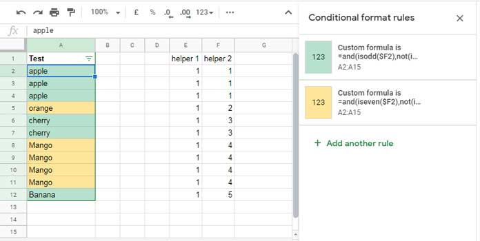
Here, in the example screenshot (GIF image) below, there is a filtered list in column A.

Similar items have been grouped by sorting. Also, I’ve set alternating colors for groups of data (rows).

See what happens when I filtering out the row containing “Orange”. The alternating colors of groups get refreshed, right? This post describes the same.

Let me help you to sort out alternating colors for the group of rows and associated filter issues in Google Sheets.

Steps to Sort Out Filter Issue Associated with Alternating Colors for Groups in Google Sheets

First of all, make your list in column A in ‘Sheet1’. For testing, you can use the same above values (fruit data) as my explanation below will be based on that.

In the next step, label cell E1 as “Helper 1” and cell F1 as “Helper 2”.

In cell E2, copy-paste the following formula and drag down until the last row that contains a value in column A (until E12 as per my sample list in column A).

=subtotal(103,A2)

Note: I will explain this formula and the following formulas under a separate subtitle at a later stage of this tutorial.

I will tell you what formula to use in helper column 2 (in cell F2). Before that “Add a new Sheet” (a second tab) and name it ‘Helper Tab’.

In that, we only require 3 columns. In cell A1 of the ‘Helper Tab’ enter the below Filter formula.

=filter({row(Sheet1!A1:A),Sheet1!A1:A},Sheet1!E1:E=1)

This will populate some values in Column A and B in the ‘Helper Tab’

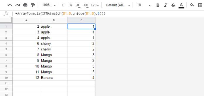
In C1 in the same tab, key this formula in.

=ArrayFormula(IFNA(match(B1:B,unique(B1:B),0)))

Go back to ‘Sheet1’ and in cell F2 enter the below Vlookup formula.

=ArrayFormula(IFNA(vlookup(row(A2:A),'Helper Tab'!A1:C,3,0)))

In ‘Sheet1’ select the range A2:A. Then go to Conditional Formatting (Format menu).

There under the custom formula field, enter the below rules one by one.

Rule 1:

=and(isodd($F2),not(isblank($F2)))

Rule 2:

=and(iseven($F2),not(isblank($F2)))

Don’t forget to choose two different colors for the above two rules.

I hope you have completed all the steps above. Then let’s test my workaround!

Hide the row # 5. The conditional formatting will correctly adjust/refresh the alternating colors.

This way you can sort out alternating colors for groups and filter issues in Google Sheets.

Can You Explain the Purpose of the Helper Columns (Formulas) and Helper Tab?

Let’s start with helper column E in ‘Sheet1’, then ‘Helper Tab’ and then helper column F again in ‘Sheet1’.

Subtotal as Counta

The Subtotal formula which uses function number 103 in cell E2 is equal to Counta. But there is one difference. The formula counts cell A2 if the row is visible.

Since we have copied this formula to E3:E12, the formulas would return 1 in all the rows except the hidden rows, if any.

What about the rows which are hidden?

If any of the rows are hidden in the range, the corresponding cell value in column E will be 0.

We will use this column as the criteria column in a Filter formula in the ‘Helper Tab’.

Helper Tab Formula 1 – Filter

The ‘Helper Tab’ A1 has a Filter formula that filters visible items from the list in ‘Sheet1’ column A.

Along with the list, the formula returns the corresponding row numbers. This row numbers will come in handy later.

The criterion in Filter is Sheet1!E1:E=1 which means if the row is not hidden.

Helper Tab Formula 2 – Array Formula for Alternating Colors for Groups

In the same ‘Helper Tab’, there is one more formula in cell C1. That formula can be used to conditional format alternating colors for Groups using ISODD/ISEVEN functions but we don’t want any highlighting in this ‘helper Tab’

The array formula in cell C1 assigns sequential numbers based on groups.

If you ask me how, here is a very detailed tutorial – Assign Same Sequential Numbers to Duplicates in a List in Google Sheets. Only follow the link if you have enough free time right now.

If we want we can highlight alternating colors for groups in column B in this ‘Helper Tab’.

How?

Since the numbers in column C are sequential, these numbers are like odd, even, odd, even… patten for groups.

We can highlight all the rows containing odd numbers with one color and even numbers with another color.

This is a helper tab and we don’t want any highlighting on this tab. Then?

Vlookup in Sheet1 – Assing Sequential Numbers to Visible Rows

The Vlookup formula in cell F2 (in ‘Sheet1’) uses row numbers as search keys and match the same row numbers in column A in ‘Helper Tab’.

If matches it will return the sequential numbers from ‘Helper Tab’ column C. So there will always be correct sequential numbers (un-broken) in column F in ‘Sheet1’.

That means if you hide any row, that won’t break the sequence of numbers in column F. Because ‘Helper Tab’ doesn’t contain that row.

Our conditional formatting ISODD and ISEVEN rules, I mean alternating colors for Groups, are based on this column F. So filter won’t have any effect on the highlighting.

This way you can get alternating colors for groups without filter issues in Google Sheets.