


Do you know how to allow only n digits in a cell/cell range in data validation in Google Sheets?
Say you want to restrict the entry of a number in a cell to 10 digits or a maximum of 10 digits.
If you think you can use a custom formula around ISNUMBER and LEN for this, it won’t work in all cases.
I haven’t get it. Can you explain, please?
Assume the cell in question (data validation) is B1. To allow only n (read 10) digits in data validation, you can use the below formula.
=and(isnumber(B1),len(B1)=10)For a maximum of 10 digits, change =10 to <=10.
To use this formula, open the data validation dialog box (menu command) from Data > Data validation > Criteria > Custom formula is.
Insert the above AND, ISNUMBER, and LEN combo formula in the blank field there.
What if I want to allow leading zeros, such as a phone number starting with 0, with the numbers and limit the number of digits?
When it comes to numbers, leading zeros (0 prefixes) make differences in spreadsheet formulas/rules.
Because, most probably, you may want to change the format from number to text.
So we may require a formula that will only accept the digits from 0 to 9 either in number or text format.
We can use Regexmatch here.
Regexmatch to Allow Only N Digits and Leading Zeros in Data Validation
You may replace n in the following formulas with the number you want. As per our example, replace it with 10
Formula # 1 – Permit Only N digits (with or without leading zeros)
=regexmatch(B1&"","^[0-9]{n}$" )Formula # 2 – A Maximum of N Digits (with or without leading zeros)
=regexmatch(B1&"","^[0-9]{0,n}$" )Here are the necessary settings within the data validation dialog box.
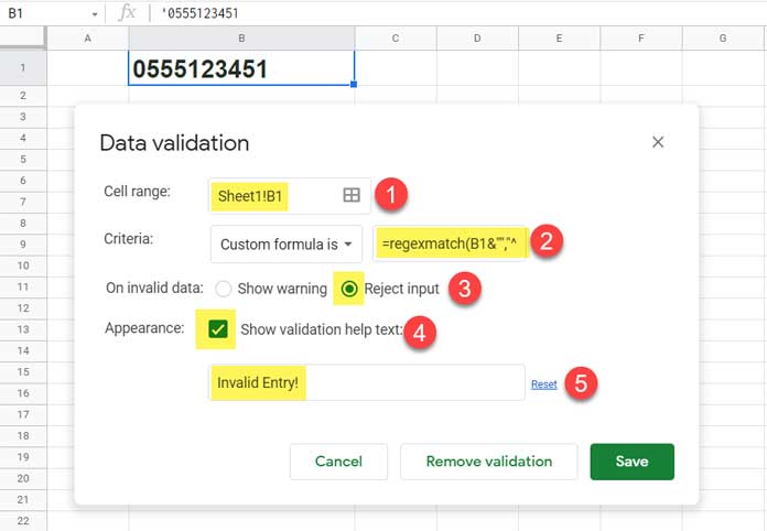
To open the above dialog box, go to the Data menu.
Settings (as per the screenshot above):-
- It’s the cell or cell range in which you want to apply the above data validation rules.
- Copy-paste either of the above formulas. You may replace cell reference B1 in the formula with the selected cell in point # 1 above.
- If you use the first Regexmatch formula, it will allow the user to enter only a number with n digits. If you go ahead with the second one, it will permit the user to enter only a number with a maximum of n digits. Please note that the formulas support numbers formatted as text to extend support to leading 0s.
- Show a warning/help text when trying to enter a number that violates the set rule in that cell.
What about a Cell Range?
You want, most probably, to apply the above regex data validation rule to a cell range/array.
That will help you create a proper and valid list in your Google Sheets, such as a list of phone numbers, product codes, employee IDs, etc.
There are no major changes either in the formula or in the data validation settings!
The two changes required are as follows.
As per the above image, in point # 1 within the dialog box, replace Sheet1!B1 with the corresponding cell range.
E.g.:
To allow only n digits in data validation for the range C1:C10 in the “Test Data” sheet, change Sheet1!B1 to 'Test Data'!C1:C10.
In the formula, you should change B1 to C1.
That’s all. Thanks for the stay. Enjoy!
Resources:
- Data Validation – How Not to Allow Duplicates in Google Sheets.
- Proper Way to Use Currency Formatting in Data Validation Drop-Down in Google Sheets.
- Reject a List of Items in Data Validation in Google Sheets.
- Data Validation to Enter Values from a List as per the Order in the List.
- Create a Drop-Down to Filter Data From Rows and Columns.
- Highlight Cells with Error Flags in the Drop-down in Google Sheets.
- Relative Reference in Drop-Down Menu in Google Sheets.
- Split Number to Digits in Google Sheets.
- Filter (Also Highlight) Unique Digit Numbers in Google Sheets.