By default, the SUMIF function in Google Sheets ignores blank cells in the criteria range, even if the corresponding sum_range values are filled. But what if you want to treat blank cells in the criteria range as if they hold the value from the cell above?

In this tutorial, you’ll learn how to include adjacent blank cells in a SUMIF range in Google Sheets. We’ll use a dynamic formula that fills blank cells virtually with the value above before performing the conditional sum.

The Problem with SUMIF and Blank Cells

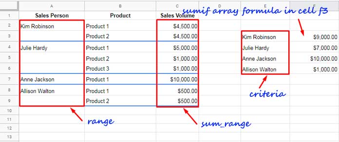
Here’s a typical scenario. Consider the following dataset:

If you try to sum values where the name is “Kim Robinson” using:

=SUMIF(
   A2:A, 
   "Kim Robinson", 
   C2:C
)

You’ll get 4500 because it only includes rows where the name cell explicitly says “Kim Robinson.” The blank rows are skipped—even though they belong to the same person.

The Solution: Fill Blanks on the Fly

To solve this, we virtually fill down the blank cells using a LOOKUP formula inside SUMIF.

Here’s the final formula that includes adjacent blank cells in the SUMIF range:

=SUMIF(
   ARRAYFORMULA(LOOKUP(ROW(A2:A), ROW(A2:A)/(A2:A<>""), A2:A)), 
   "Kim Robinson", 
   C2:C
)

What It Does:

• LOOKUP(...) fills blank cells in column A with the last non-blank value above.
• SUMIF(...) then sums values from column C based on these filled-in values.

You can learn more about how this LOOKUP approach works in my tutorial: Fill Blank Cells with Values from the Cell Above in Google Sheets.

Alternatively, you can use this modern SCAN formula to achieve the same result dynamically:

=SUMIF(
   SCAN(, A2:A, LAMBDA(accu, val, IF(val="", accu, val))), 
   "Kim Robinson", 
   C2:C
)

I’ve explained how the SCAN method works in that same tutorial as well.

Example 1: Criteria in a Separate Column

You can also adapt this for a list of names in a separate column (e.g., E2:E5), like so:

=ARRAYFORMULA(
   SUMIF(
      LOOKUP(ROW(A2:A), ROW(A2:A)/(A2:A<>""), A2:A), 
      E2:E5, 
      C2:C
   )
)

This version sums the amount column for each unique name in your criteria list, even if the names appear in a range with blanks.

Why This Works

The key is LOOKUP—it dynamically replaces blanks with the last seen non-blank entry, creating a temporary version of the range with no blanks. This lets SUMIF operate as if the data had already been cleaned.

Summary

If your dataset has blank cells in the criteria range and you’d like to treat them as if they repeat the previous value, use LOOKUP with ROW inside SUMIF. This lets you:

• Avoid manually filling blanks
• Work with dynamic ranges
• Get accurate totals without modifying your original data

Related Reading

• How to Use SUMIF in Merged Cells in Google Sheets
• Multiple Criteria SUMIF Formula in Google Sheets
• How to Sum Every Nth Row in Google Sheets
• How to Use Dynamic Ranges in SUMIF Formula in Google Sheets
• Use MMULT Instead of SUMIF for Conditional Totals in Sheets
• How to Perform a Case-Sensitive SUMIF in Google Sheets