You might want to count the number of words in a cell in Excel as part of data validation or conditional formatting. If you are a content creator using Excel for keyword count, you might also be interested in counting the words as part of your workflow.
For counting words in a cell in Excel, you can use two types of formulas. One is a workaround that works with all versions of Excel, and the other is a genuine word count formula, which requires Excel 365.
Can we use them in cell ranges as well? Yes, certainly.
Word Count Using a Workaround in Excel
You should follow this Excel word count formula if you are not using Excel for Microsoft 365.
Generic Formula:
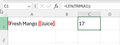
=IF(cell<>"", LEN(TRIM(cell))-LEN(SUBSTITUTE(cell," ",""))+1,"")For counting the number of words in the text in cell A1, you can use the following formula in cell B1:
=IF(A1<>"", LEN(TRIM(A1))-LEN(SUBSTITUTE(A1," ",""))+1,"")How does this formula work?
Formula Breakdown:
Let’s assume the text in cell A1 is ” Fresh Mango Juice “, which contains three words: “Fresh,” “Mango,” and “Juice.” It contains leading, trailing, and extra spaces, though.
Part 1:
LEN(TRIM(A1))This will return 17, the length of the string in cell A1 after removing leading, trailing, and extra spaces.
TRIM(cell)removes leading, trailing, and repeated spaces in the text in the specified cell.LENfunction returns the length of the string.
Part 2:
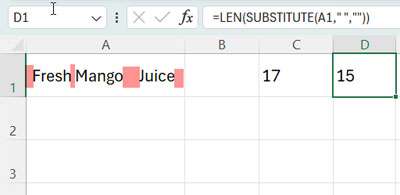
LEN(SUBSTITUTE(A1," ",""))This will return 15, i.e., the length of the string after removing all spaces.
SUBSTITUTE(A1," ","")replaces all spaces with null.LENfunction returns the length of the string.
Excel Word Count:
Part 1 - Part 2This returns the number of spaces in the text. We need to add 1 to this count to get the word count in that cell.
The role of =IF(A1<>"", ... ,"") is to return a blank value if the cell doesn’t contain any value.
The Genuine Word Count Formula in Excel
If you are using Excel for Microsoft 365, you can use the following formula, though the above workaround works.
Generic Formula:
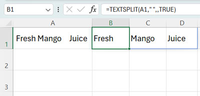
=IF(cell<>"", COUNTA(TEXTSPLIT(cell," ",,TRUE)),"")If you want to find the word count in cell A1, apply the following formula to cell B1:
=IF(A1<>"", COUNTA(TEXTSPLIT(A1," ",,TRUE)),"")Why do we call this the genuine word count formula in Excel?
The TEXTSPLIT function splits the provided text string by using a column delimiter that is ” “. The COUNTA function counts those words.
Similar to our workaround formula, the purpose of =IF(A1<>"", … ,"") is to return a blank value if the cell doesn’t contain any value.
Counting Number of Words in a Range in Excel
The above single-cell word count is usually useful in data validation and conditional formatting in Excel.
For those who are content creators, you may want to count the words in a column or multiple columns all at once.
Single Column:
Assume you want to count the words in A1:A100 in your Excel spreadsheet. If you are not using Excel in Microsoft 365, you can use my workaround formula.
In cell B1, enter the following formula:
=IF(A1<>"", LEN(TRIM(A1))-LEN(SUBSTITUTE(A1," ",""))+1,"")Drag the fill handle in the bottom right corner of cell B1 (it appears only when the cell is selected) down to cell B100.
In cell C1, enter the following formula to total the number of words:
=SUM(B1:B100)If you are using Excel for Microsoft 365, you are lucky to use the Lambda functions.
Simply enter this formula in cell B1:
=SUM(MAP(A1:A100,LAMBDA(val,IF(val<>"",COUNTA(TEXTSPLIT(val," ",,TRUE)),""))))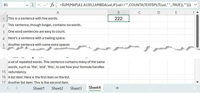
Two Column:
The above two formulas are flexible enough to count words in multiple columns in an Excel spreadsheet, both in newer and older versions.
For data in columns A and B, you can use the following formulas.
Drag Down Formula:
Apply this formula in cell C1 and drag it down as far as needed, then sum the results in cell D1:
=IF(A1&B1<>"", LEN(TRIM(A1&" "&B1))-LEN(SUBSTITUTE(A1&" "&B1," ",""))+1,"")Dynamic Array Formula:
As before, simply enter this formula in cell C1:
=SUM(MAP(A1:B100,LAMBDA(val,IF(val<>"",COUNTA(TEXTSPLIT(val," ",,TRUE)),""))))Resources
Here are a few related resources:


