When you have two tables containing an ID column in each, you can combine these tables into a third table in Excel.
For instance, consider an employee data table comprising employee ID, first name, last name, department, and position.
Additionally, there’s a second table containing employee ID, date, and the amount of advance given.
How do we match the records in the second table and append them to the first table to create a third table?
VLOOKUP or XLOOKUP wouldn’t be ideal for combining two tables because they only return the first or last matching record when an employee has multiple entries in the second table.
This necessitates the need for a custom formula to combine two tables in Excel. I’ve developed a dynamic array formula in Excel for this purpose.
The formula is straightforward and to use with tables of any number of columns, requiring minimal adjustments, which I will explain clearly.
Table 1: Employee Data
I have the following data in the range Sheet1!A1:E7 in my Excel 365 spreadsheet.
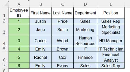
The first column contains the employee IDs, which are unique identifiers when combining this table with the second table.
After we join this table with the second table, the formula should retain all the records in this table, i.e., employee IDs, first names, last names, departments, and positions.
Table 2: Advance Given
In the same workbook, within Sheet2, the data in the range A1:C6 is as follows:
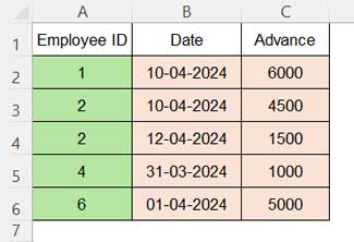
The first column contains employee IDs, the second column contains dates of advance given, and the third column contains the amounts of advance given.
When paying advances to employees, we simply note their ID, the date of payment, and the payment amount. This process saves time.
When we require employee names and other data, we can use the IDs in Table #2 as search keys and use Table #1 as the lookup range in VLOOKUP or XLOOKUP. This fetches the necessary data.
However, since we are combining this table with the first table, we will have a third dataset with all employee data and advance details against those employees who have taken advance.
This is where the dynamic array formula comes into play, as it efficiently combines the two tables.
Prerequisites for Combining Two Tables
The only requirement you should comply with to combine two tables is the position of the ID column. It should be the first column in the tables.
As you can see in my tables, employee IDs are the unique identifiers, and they are in the first column of the tables.
Actually, the formula can take the ID column from any position in the range. However, you may need to reorder the columns in the combined table, which might complicate things for novice users. So, let’s keep the first column as the unique identifier column in both tables.
Dynamic Array Formula for Combining Two Tables in Excel
The formula may seem a bit complex at first glance. However, it’s simple to use if you follow my tips. Let’s explore the formula for merging two tables and their output.
Formula in cell A1 (Sheet3):
=LET(tableA, Sheet1!A1:A7& "|"& Sheet1!B1:B7&"|"& Sheet1!C1:C7&"|"& Sheet1!D1:D7&"|"& Sheet1!E1:E7, keyA, Sheet1!A1:A7, nA, 5, tableB, Sheet2!A1:C6, keyB, Sheet2!A1:A6, nB, 3, keys, DROP(REDUCE("", keyA, LAMBDA(accu, val, VSTACK(accu, IFNA(HSTACK(ROW(val), IFERROR(FILTER(tableB, keyB=val), "")), ROW(val))))), 1), r, XLOOKUP(CHOOSECOLS(keys, 1), ROW(A1:A7), tableA), d, "|", n, nA, split, TEXTBEFORE(TEXTAFTER(d&r&d, d, SEQUENCE(1, n)), d, 1), fnl, IFERROR(IFERROR(split*1, split), ""), IFNA(HSTACK(fnl, CHOOSECOLS(keys, SEQUENCE(1, nB-1, 3))), ""))Merged Table:
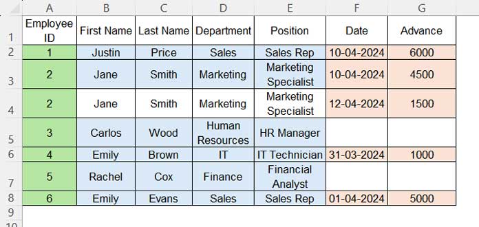
The above formula in cell A1 in Sheet3 combines the tables in Sheet1 and Sheet2. Here are the required changes you may need to make to adapt this formula in your Excel table merging.
Please refer to the highlighted names in the formula where you need to make the changes.
Change 1:
tableA – represents the first table range.
Specify each column and combine them with a pipe delimiter as shown below:
Sheet1!A1:A7 & "|" & Sheet1!B1:B7 & "|" & Sheet1!C1:C7 & "|" & Sheet1!D1:D7 & "|" & Sheet1!E1:E7Change 2:
keyA – represents the key (unique identifier) column in the first table.
As per our Table 1, it is specified as Sheet1!A1:A7
Change 3:
nA – represents the number of columns in the first table.
As per our Table 1, specified as 5
Change 4:
tableB – the second table range
As per our Table 2, specify as Sheet2!A1:C6
Change 5:
keyB – key (unique identifier) column reference in the second table
As per our Table 2, specify as Sheet2!A1:A6
Change 6:
nB – number of columns in the second table
As per our Table 2, specify as 3
With these changes, you can combine two tables in Excel.
Conclusion
We can merge two tables in several ways, specifically using left join, right join, inner join, and full join. Our Excel dynamic array formula falls under the category of left join.
Related: Master Joins in Google Sheets (Left, Right, Inner, & Full) – Duplicate IDs Solved
Can we also use this formula for right, inner, and full join?
Let me clarify their differences briefly and then provide the answer.
| Join Type | Description |
| Left | Returns all records from Table A and the matching records from Table B. |
| Right | Returns all records from Table B and the matching records from Table A. |
| Inner | Returns only the records having matching values in Table A and Table B. |
| Full | Returns all records from Table A and Table B. |
Our dynamic array formula for combining two tables in Excel can be used for left or right join. You need to use Table B references instead of Table A references and vice versa.
For inner and full join, you may require using helper columns to add or remove values from the left joined table using functions like FILTER and XMATCH.


