


Do you want to illustrate your job schedule in a flash within a Google Spreadsheet?
Using my custom GANTT_CHART named function, you can now create Gantt Charts in a flash in Google Sheets.
It’s an array function. So capable of covering all the tasks in one go!
It just requires the following inputs.
- Tasks’ start date range.
- Tasks’ end date range.
- Project start date (period from).
- Project end date (period to).
- Status range (to return bars with different colors based on the progress of the tasks).
The GANTT_CHART array function will take care of the rest!
Additionally, you can use a child function to draw the timescale at the top of the bar area.
Syntax and Arguments of the GANTT_CHART Custom Named Function
Syntax:
GANTT_CHART(start_date_range, end__date_range, from, to, status)Arguments:
start_date_range: The start date range of tasks.
end__date_range: The end date range of tasks.
from: Timescale start date. It can be either a cell reference or a hard-coded date.
to: Time scale end date. It can be either a cell reference or a hard-coded date.
If you use the project start date in from and the project end date in to, the formula will return bars for all the tasks.
If you want to view the bars of tasks that fall in a particular period, use those start and end dates in from and to arguments.
status: The status column range against tasks.
It controls the color of the bars. It is one of the salient features of my custom GANTT_CHART function in Google Sheets.
Here are the supported texts in the status column and corresponding bar colors.
Use the following four statuses in the status column when you want to illustrate the progress of your project. Please scroll down and see example # 1 below.
Table 1
| Status | Bar Color |
| Upcoming | Orange |
| In progress | Blue |
| Hold | Red |
| Complete | Green |
Sometimes, you may require two bars for each task – One for scheduled progress and another for actual progress.
In that case, use the below two statuses. Please scroll down and see example # 2 below.
Table 2
| Status | Bar Color |
| Sch | Blue |
| Actual | Green |
My custom GANTT_CHART function will return grey colors for all the other texts in the status range.
I don’t have a status column. What should I do?
Refer to any range. The function will return grey-colored bars. Please scroll down and see example # 3 below.
Prerequisites (Formatting)
The formula requires 60 merged columns in each row. So that it can properly return all the bars.
For example, if the bar area starts from row # 4 in column F, you must merge F4:BM4, F5:BM5, F6:BM6, and so on. Please scroll down and see screenshot # 1.
To merge columns, select F4:BM4 and apply Format > Merge cells > Merge all.
Repeat the same for other rows below until you reach the last row containing the task.
To get the timescale on the top of the bar area, use my custom TIMESCALE() child function.
For example, use the said function-based formula in cell F3.
We will see both of these in detail in the examples below.
To get the functions, you may make a copy of my example sheet below and follow the instructions in my Named Function tutorial to import them.
How to Use the GANTT_CHART Function in Google Sheets
Here are three examples.
Example # 1:
The status column (E4:E) contains the texts as per table 1 above.
=GANTT_CHART(B4:B,C4:C,"15/11/2021","31/03/2022",E4:E)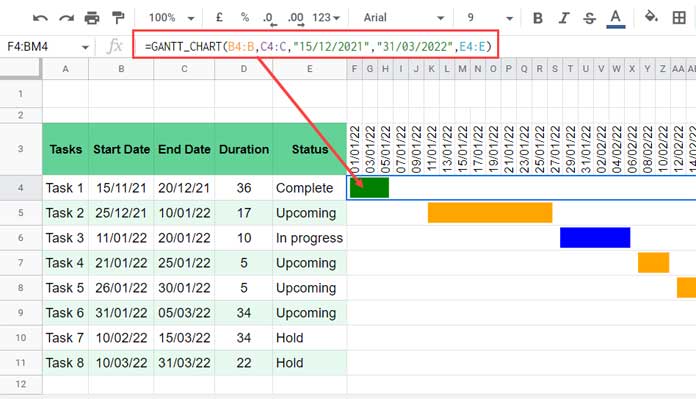
In the above GANTT_CHART function example in Google Sheets, B4:B is the start_date_range, C4:C is the end_date_range, 15/11/2021 is from, and 31/03/2022 is to, and E4:E is the status.
Note:- You feel free to enter the from and to dates in any two cells and refer to them in the formula.
The formula in F4 returns the bars for all the tasks that fall in the period from 15/11/2021 to 31/03/2022.
Do not copy the formula down! GANTT_CHART is an array function that returns bars in all rows in the range in one go.
What about the TIMESCALE() formula in cell F3?
We will come to that later.
Example # 2:
The status column (E4:E) contains the texts as per table 2 above.
=GANTT_CHART(B4:B,C4:C,"15/11/2021","31/03/2022",E4:E)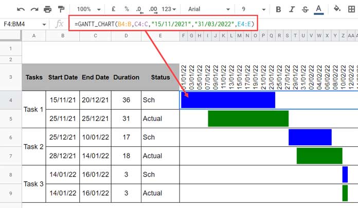
Here each task has two rows – one for scheduled dates and the other for actual dates.
Example # 3:
This time there is no status column in the table. So used A4:A (any column) as the status column. So all the bars are in grey color.
=GANTT_CHART(B4:B,C4:C,"15/12/2021","31/03/2022",A4:A)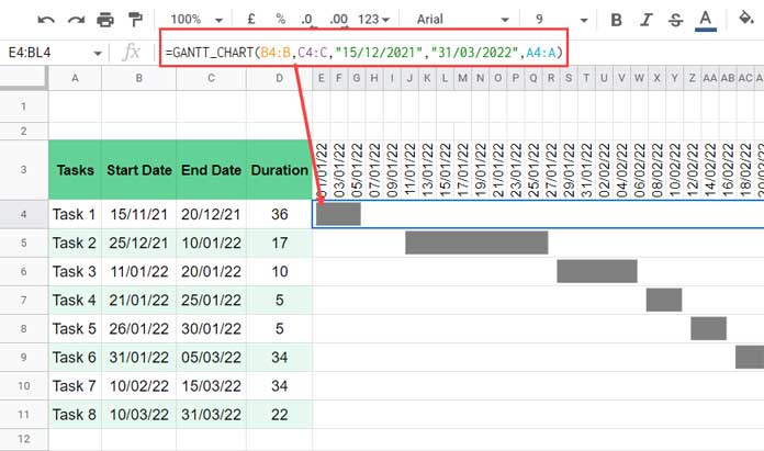
TIMESCALE Child Function and Its Usage
As you can see, the GANTT_CHART named function is so easy to use in Google Sheets.
Now what we lack is a function that returns the timescale in F3:BM3.
Here it is!
=TIMESCALE("01/01/2022","31/03/2022")The above array formula in cell F3 returns the proper timescale for the chart.
Take the from and to dates from the GANTT_CHART formula to input within the TIMESCALE() child function.
They should match.
Syntax:
TIMESCALE(from, to)That’s all. Thanks for the stay. Enjoy!
Resources
- Create GANTT Chart in Google Sheets Using Stacked Bar Chart.
- Create Gantt Chart Using Formulas in Google Sheets.
- Create a Gantt Chart Using Sparkline in Google Sheets.
- Split a Task in Custom Gantt Chart in Google Sheets.
- Multi-Color Gantt Chart in Google Sheets.
- Flexible Timescale for Gantt Chart in Google Sheets.
- Days Remaining in Gantt Chart in Google Sheets.
- Date Filter in Gantt Chart in Google Sheets.