How to Split a Task in Gantt Chart in Google Sheets

Need to split a task in a Gantt chart in Google Sheets? If a task gets paused midway—maybe due to bad weather at a construction site or a change in plans—you might want to show that gap in your chart. That’s exactly what this tutorial is about.

We’ll work with a conditional-format-based Gantt chart, which is simple and fully formula-driven. You won’t need charts or graphs—just smart formatting.

Table of Contents

Quick Note on Gantt Chart Options in Google Sheets

There are a few ways to build Gantt charts in Sheets. This post focuses on the one made using conditional formatting. I’ve already covered how to build that kind of Gantt chart in this post, so I’ll quickly run through the key parts again—mainly because we’ll be reusing that setup to split the task bars.

But just so you know, here are two other ways to create Gantt charts in Sheets:

Using a stacked bar chart
Using the SPARKLINE function

They work too, but the conditional format method is lightweight and flexible—perfect for this use case.

Gantt Chart Using Conditional Formatting

Let’s start with a basic Gantt chart setup using conditional formatting.

To make it work, you’ll need:

A Task Name column (let’s say column A)
A Start Date column (column B)
An End Date column (column C)
A row of dates (the timescale) going across—say, D2:AB2

These dates will act as the timeline over which task bars appear.

A basic Gantt chart in Google Sheets using conditional formatting to show task bars across a weekly timescale

Creating the Timescale

Here’s a formula you can use in cell D2 to generate a weekly timeline starting from 6-Jan-2020 and covering 25 weeks:

=SEQUENCE(1, 25, DATE(2020, 1, 6), 7)

That’s:

25 columns (weeks)
Starting from 6-Jan-2020
Incremented by 7 days each time

Want to switch to daily or monthly? Just change the step value from 7 to 1 or 30.

This setup is all you need to show the task bars—and yes, to split tasks in the Gantt chart too.

Note: While this example uses a weekly schedule, it’s usually better to go with a daily timescale (step value 1) if your tasks or splits are short. That way, the bars and interruptions show up more clearly in the Gantt chart.

Apply the Conditional Formatting Formula

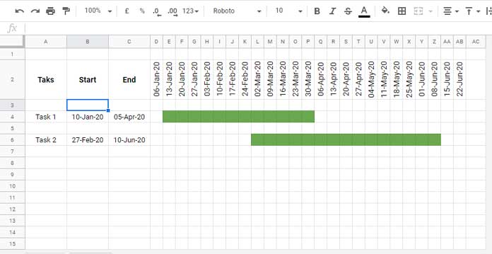
Let’s say your task data starts in row 3 and goes down to row 14, and your timeline runs from column D to AB. That means your formatting range is D3:AB14.

Here’s the custom formula to highlight cells between the start and end dates:

=AND(D$2 >= $B3, D$2 <= $C3)

Just select the range D3:AB14, open Format > Conditional formatting, and paste the formula.

Set your fill color (gray, blue, whatever works). Now you’ve got your basic Gantt chart bars in place.

Google Sheets conditional formatting panel showing a custom formula applied to create Gantt chart bars

Add a new task in row 8 or 10 or 14—the formula still works. No need to change anything.

Split a Task in Your Gantt Chart

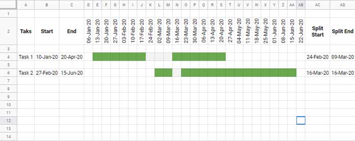
Let’s say Task 1 starts on 10-Jan-2020 and ends on 05-Apr-2020, but there’s a 3-week break from 24-Feb-2020 to 09-Mar-2020. We want the chart to:

Blank out that 3-week gap in the bar
Extend the task bar by 3 weeks at the end

Here’s how to do that.

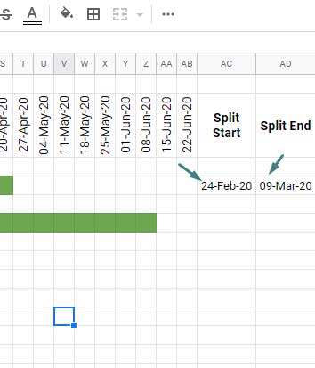
Step 1: Add Split Start and End Columns

We’ll add two extra columns—for the split start and split end dates. Let’s say columns AC and AD.

So in row 4 (Task 1):

AC4: 24-Feb-2020
AD4: 09-Mar-2020

This tells Sheets where the gap in the bar should be.

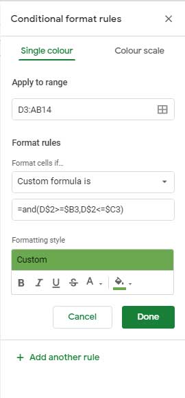
Split start and end date columns added to a Gantt chart for showing task interruptions

Step 2: Add a Rule to Remove the Split Segment

Now we’ll add another rule to remove the bar in that gap.

Select the same range: D3:AB14
Go to Format > Conditional formatting
Click + Add another rule
Use this formula:

=AND(D$2 >= $AC3, D$2 <= $AD3)

Set the fill color to white (or the background color of your sheet)

You’re basically telling Sheets: “If the date falls within this split range, remove the bar.”

Step 3: Reorder the Rules

In the conditional format rules panel, drag this new rule above the original one.

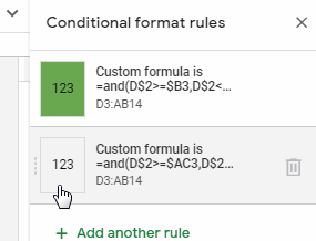
Reordering conditional format rules in Google Sheets to apply the split task logic correctly

Why? Because format rules work in order—the top one gets applied first. By putting the “remove bar” rule first, it overrides the color in the split range.

Step 4: Adjust the Task End Date

To make room for the split, extend the end date.

Original end date in C4: 05-Apr-2020
Add 3 weeks → new end date: 20-Apr-2020

That works because the next bar in the timescale would begin on 27-Apr-2020, so ending on 20-Apr-2020 keeps the task bar accurate without overshooting.

Split tasks displayed in a conditional-format-based Gantt chart in Google Sheets, showing gaps and extended bars

Add a Split for Another Task

Let’s split Task 2 for just one week:

AC6: 16-Mar-2020
AD6: 16-Mar-2020
Extend the end date in C6 by one week—say to 15-Jun-2020

You don’t need to add a new formatting rule for each task—just enter the split start and end dates in the right columns, and the existing rule will take care of the rest.

How to Remove a Split from a Task

Changed your mind?

Just delete the split start/end dates in AC and AD
Restore the original end date in column C

Your Gantt chart goes back to normal.

Final Gantt Chart with Split Tasks

Now you can clearly show interruptions or multi-phase work in your Google Sheets Gantt chart. Whether it’s construction, design, or development—splitting tasks helps you communicate project progress better.

And all of this works using just conditional formatting formulas—no charts needed.

Sample Gantt Chart