


![Excel Hotel Room Availability Template [Free]](https://infoinspired.com/wp-content/uploads/2024/05/Excel-Hotel-Room-Availability-Template-218x150.jpg "Excel: Hotel Room Availability and Booking Template (Free)")


There are so many benefits of using Filter with Vlookup result columns in Google Sheets.
To name a few, it will help you filter out blanks, remove unwanted single or multiple values from the lookup row, and apply comparison operators.
We will discuss them in this new Google Sheets tutorial.
Introduction
In my opinion, earlier, Vlookup in Google Sheets was far superior in comparison to its Excel sibling. You feel free to agree or disagree with it.
The possibility of tweaking Vlookup to meet our lookup requirements is endless in Google Sheets. There are three main reasons for this.
- The function accepts expressions in all the arguments.
- The availability of array functions like Filter, Sort, Query that we can use within Vlookup or outside as a combination (to learn these functions, please refer to my function guide).
- Google Sheets has an ArrayFormula function instead of the Ctrl+Shift+Enter legacy array formula in Excel to work with arrays.
As a side note, we will make the best use of the above second feature to filter Vlookup result columns in Google Sheets.
The above point # 3 was the game-changer.
Because, in Google Sheets, we could make virtual arrays using Curly Brackets. That offered endless possibilities of tweaking the range to Lookup.
But later, Excel has caught up by introducing XLOOKUP and dynamic array functions such as Filter and Sort (though not in all versions).
Now Excel is also competent enough to meet all lookup requirements.
You May Like: Comparison of Vlookup Formula in Excel and Google Sheets.
Sample Data
To filter a Vlookup result, we must know how to get values from all the columns in the lookup row.
I have already explained the same here – How to Return Multiple Values Using Vlookup in Google Sheets?
Want an example? Then here you go!
Master Formula:
=ArrayFormula(vlookup(A1,A4:H9,column(B3:H3),0))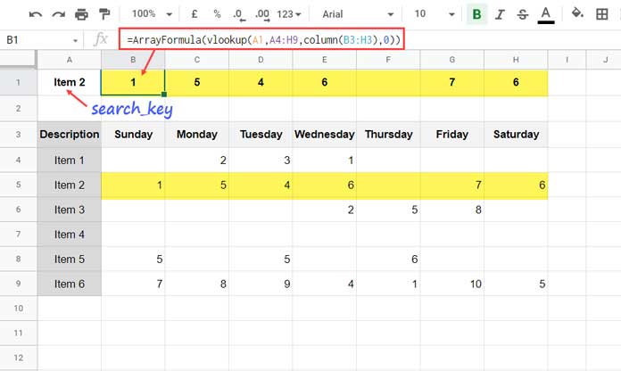
search_key – A1, which is the “Item 2”
range – A4:H9 (the range to lookup for the search_key in the first column).
index – column(B3:H3), which is columns 2 to 8.
The above formula returns a 7 column result.
See below how we can filter Vlookup result columns in Google Sheets to meet our different requirements.
Example to Filtering Vlookup Result Columns in Google Sheets
Please find a couple of formula examples under three sub-titles below.
Filter Out Blanks from Vlookup Result Columns
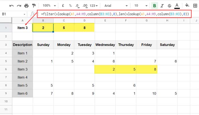
If you repace the search_key in cell A1 with “Item 3”, the master formula would return the below result.
| 2 | 5 | 8 |
Let’s Filter these Vlookup result columns to remove the blank cells (ArrayFormula removed as it’s not required with Filter).
=filter(
     vlookup(A1,A4:H9,column(B3:H3),0),
     len(vlookup(A1,A4:H9,column(B3:H3),0))
)
This is useful when you want to get result from the first ‘N’ non-blank columns in Vlookup. For that just include Array_Constrain with it.
=array_constrain(
     filter(
        vlookup(A1,A4:H9,column(B3:H3),0),
        len(vlookup(A1,A4:H9,column(B3:H3),0))
     ),1,N
)
Replace ‘N’ with 1 to get the first value, 2 to get the first two values, and so on.
Earlier, we were using a different formula that is only capable of returning the first non-blank value after a vertical lookup. Here is that tutorial – Move Index Column If Blank in Vlookup in Google Sheets.
That was a nested Vlookup formula.
Applying Comparison
The Filter Vlookup combination has several advantages, and here is the next one that uses a comparison operator.
Let’s interpret the contents of the above table as below.
A4:A9 – sales items.
B4:H9 – sales quantities of items in A4:A9 from Sunday to Saturday.
Assume you want to lookup “Item 6” in column A and return the sales values less than 5.
=filter(
     vlookup(A1,A4:H9,column(B3:H3),0),
     vlookup(A1,A4:H9,column(B3:H3),0)<5
)
It will do that.
Filter Vlookup Result Columns in Google Sheets to Remove Unwanted Values
Actually, in the above two examples, we have already learned to remove unwanted values.
To further fine-tune the result, we can use other comparison operators or the Regex.
In the below three formula examples, you may please pay attention to the third one that uses regular expression.
Example # 1
To Filter Vlookup result columns for the value not equal to 5.
=filter(
     vlookup(A1,A4:H9,column(B3:H3),0),
     vlookup(A1,A4:H9,column(B3:H3),0)<>5
)
Example # 2
To only to return the value 5.
=filter(
     vlookup(A1,A4:H9,column(B3:H3),0),
     vlookup(A1,A4:H9,column(B3:H3),0)=5
)
Example # 3
It is more advanced.
We can use Regexmatch to filter Vlookup result columns using multiple conditions. This formula would only return the values 1 and 10.
=filter(
     vlookup(A1,A4:H9,column(B3:H3),0),
     regexmatch(vlookup(A1,A4:H9,column(B3:H3),0)&"","^1$|^10$")
)
If the result columns contains text, replace 1, 10 with corresponding strings.
You can add more conditions by separating them with the pipe delimiter like ^apple$|^orange$|^banana$.
To return the values that are not equal to 1 and 10 after a Vlookup, use the FALSE Boolean.
=filter(
     vlookup(A1,A4:H9,column(B3:H3),0),
     regexmatch(vlookup(A1,A4:H9,column(B3:H3),0)&"","^1$|^10$")=FALSE
)
Related: Regexmatch in Filter Criteria in Google Sheets.
Filtering Vlookup Result Columns and N/A Error
All the above formulas may return #N/A error in two cases. That is (1) when the Vlookup search_key is not present in the first column in the range or (2) when the Filter doesn’t find a match.
Assume the value in cell A1 is “Gold.” There is no such item in A4:A9.
So the Vlookup will return seven #N/A errors as we use multiple index (output) columns in the formula. If you use Filter with Vlookup, you will possibly see only one error value.
When using Example # 2 formula above and the condition/criterion in cell A1 is “Item 4”, the Filter will return the above error. It is because the condition is not matching in the Vlookup result columns.
To remove such errors and get a custom value, wrap the outer formula with IFNA.
It would be like;
=ifna(formula,"message")That’s all. Thanks for the stay. Enjoy!