


Similar to SQL you can communicate with a database table-like array, using the DMIN function in Google Sheets. All database functions in Google Docs Sheets are meant to do so.
Purpose:
The DMIN formula in Sheets can return the minimum value from a database table-like array using a SQL-like query.
You may be unfamiliar with the term database table-like array which I have used above, right?
It’s of course data or you can say records arranged in rows. But, similar to a database table, the first row in the range must contain the labels representing values in each column.
Are you still in a dilemma? I hope the following example can help you.
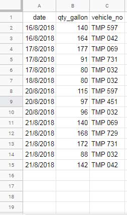
The following sample data shows the diesel consumption/filling of a few vehicles in date wise. You can see that the first row of this report contains the column labels.
In this and similar data types, you can flawlessly use the database functions including DMIN.
That means if the labels are not there you can’t use any database functions in such an array. So you must either use MINIFS, MIN, SMALL or MINA to find the min value.
The Syntax of the DMIN Database Function in Google Docs Sheets:
MIN(database, field, criteria)Arguments:
database – The range containing the data to consider which complies the above-said database table-like array features.
field – The column in the database to find the min value. Use either the column label or the column number.
criteria – The condition to filter the database.
Let me elaborate on how to use the DMIN function in Google Sheets and also the criteria usage tips.
DMIN Formula Examples
Let’s consider the above same sample data. The first column contains the dates of filling the fuel, the second column contains the filled quantities in gallons, and the third column contains the vehicle numbers. See the usage tips of the criteria in this function.
DMIN Function and String Criteria in Sheets
=DMIN(A1:C15,2,{"vehicle_no";"TMP 597"})The above formula will return the minimum quantity of the fuel filled by the vehicle # “TMP 597”.
The same DMIN formula when using the condition/criterion as a cell reference:
=DMIN(A1:C15,2,E1:E2)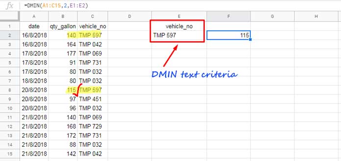
The are three types of criteria normally in use. They are text, number, and date. Other than this sometimes you may want to use the comparison operators.
I have explained above how to use the Text criteria in DMIN in Google Sheets. Now let me share you the DMIN formula that contains date as the criteria.
DMIN Function and Date Criteria in Sheets
Formula:
=DMIN(A1:C15,2,{"date";DATE(2018,8,17)})This formula filters the rows contain the date 17/08/2018 in the first column and then in that filtered data finds the min value in field 2.
See the equivalent to this formula.
=DMIN(A1:C15,2,E1:E2)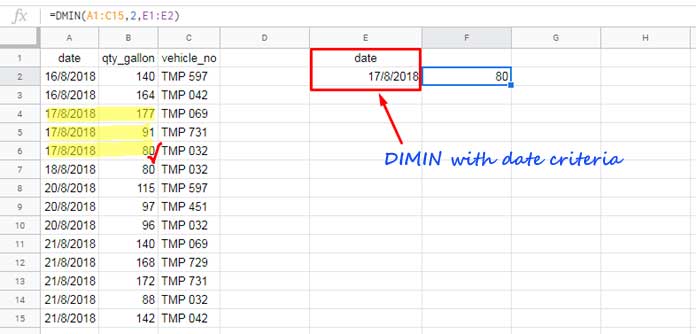
DMIN Function and Number Criteria in Sheets
There is no number column to use as the criteria field in the above sample data. There is only one column that is the field to find the min. That prompted me to consider a second sample data.
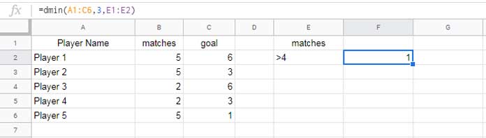
Here is a new sample data which is not realistic though. But it will be enough to explain the formula.
=dmin(A1:C6,3,E1:E2)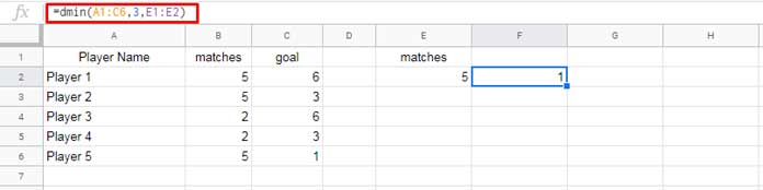
The formula returns the least number of goals conceded by any player in 5 matches. The formula can be coded as below also.
=dmin(A1:C6,3,{"matches";5})DMIN Formula with Comparison Operators
=dmin(A1:C6,3,{"matches";">"&4})When you use a comparison operator with the number criteria in DMIN, place that within double quotes and use the ampersand to join it with the number.
If it’s referred to a cell, you can directly type the criteria with the comparison operator as below.
For additional tips and tricks related to the DMIN function please check the following database functions guide related to DSUM – How to Properly Use Criteria in DSUM in Google Sheets [Chart]. You can follow the tips presented in that tutorial in DMIN too.
Before winding up one more important thing! In this tutorial, I haven’t touched the multiple criteria usage part.
I purposefully omitted that realizing it’s already posted in another tutorial related to DMAX. Needless to say, the usage tips are the same in both functions.