Why should one use the LOOKUP function in an unsorted array?
By default, you can use the Lookup function in a sorted range only. But there is a workaround to use this function in an unsorted range. That is by using a virtual search range. I’ll come to that.
What happens when one uses the LOOKUP in an unsorted array? That is important to know first. Otherwise, there is no meaning in learning the use of LOOKUP function in an unsorted array.
All the three lookup functions Vlookup, Hlookup and Lookup work well with sorted data. But the Vlookup and Hlookup work both on sorted as well as unsorted data and that you can set by entering TRUE/FALSE as the last parameter.
Leaving that aside let’s talk about the lookups in sorted data first. All the above three lookup functions return a value that is less than or equal to the search key in a sorted data called the nearest match.
All About the Lookups in Sorted Data in Google Sheets
In my examples, I am not including Hlookup. Please understand that the examples that apply to Vlookup can be applied to Hlookup also, but in a horizontal dataset only.
Lookup/Vlookup Result When Search Key is Present
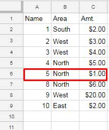
If your search key is 5, and the value 5 is there in the lookup column (it’s the first column normally) it can return 5 or value from the corresponding row.
Vlookup Formula in a Range (Search Key is Present):
=vlookup(5,A2:C,3,1)
Result: 1
Lookup Formula in a Range (Search Key is Present):
=lookup(5,A2:A,C2:C)
Result: 1
Lookup/Vlookup Result When Search Key is Not Present But Less than Value is Present
If the value 5 is not there in the lookup column the formula would return the value that is less than or you can say nearest to 5.
The same above formulas would return 5 if the data range is as below since search key 5 is not there in the lookup column (first column). It’s the nearest match.
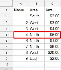
If all the values are greater than 5, then the formula returns #N/A.
If there are multiple matching values, the last matching value would be returned.
Lookup/Vlookup Result When Search Key is Present Multiple Times
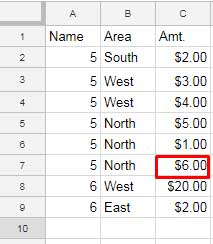
If you use the same above formulas again, it would return 6 as below. The search key 5 is available in multiple times in column A.
The formulas return the last matching value.
What Happens When We Use LOOKUP in an Unsorted Array
You have seen the formula outputs of LOOKUP in a sorted range. Now in this example, my data is not sorted.
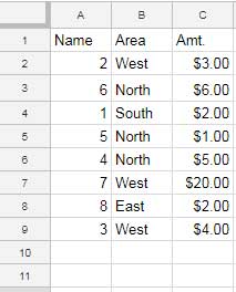
See the first column and as you can see here it is not in any order. Normally you can’t use LOOKUP in this column to get the correct output.
Hereafter I am not detailing the Vlookup as Vlookup can be used in both sorted and unsorted data by changing the last parameter in the function to TRUE/FALSE.
=lookup(5,A2:A,C2:C)
With this formula on the above dataset, I am expecting the formula to return the value 1 but it returns 5. No puzzle as the data range is not sorted.
See this new range. Here the search key 5 is available multiple times and the data is unsorted.
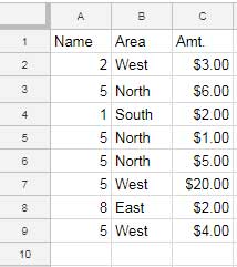
Again the formula won’t work correctly. Then why don’t you use Vlookup here?
There is a purpose of using Lookup in an unsorted data. Here you go.
What is the Purpose of Using LOOKUP Function in an Unsorted Array
Here is my answer to the question of why should one use the LOOKUP function in an unsorted array.
Here is what happens with the Vlookup in unsorted data. This is the most common Vlookup use. The 0 indicates (you can also type FALSE) the range is not sorted. This parameter is not available in Lookup.
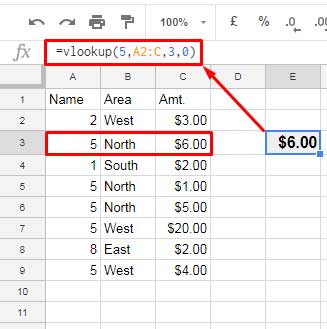
It’s all about the first match. But what I want is the last match.
For the last match, the ultimate lookup solution is Lookup. With a workaround, you can use Lookup in an unsorted data. Similarly, you can use Vlookup too. But Lookup is a more elegant solution.
How to Use Google Sheets LOOKUP Function in an Unsorted Array
We can virtually sort the data within the LOOKUP. How?
Here is the conventional lookup formula for sorted data.
=lookup(5,A2:A,C2:C)
In an unsorted data replace the search_range (here A2: A) with a virtual sorted range.
Syntax:
LOOKUP(search_key, search_range, result_range)
Here is that virtual sort_range in Lookup.
=ArrayFormula(if(len(A2:A),(1/{A2:A=5}),))
Now see the LOOKUP formula that utilizes the virtual search range that works well on an unsorted data set.
=lookup(5,ArrayFormula(if(len(A2:A),(1/{A2:A=5}),)),C2:C)
You can move the ArrayFormula to the first part.
So the final formula would be as follows.
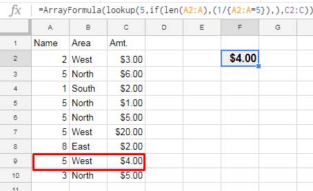
This way you can use the LOOKUP function in an unsorted Array in Google Sheets.
Can you explain to me how this virtual sort range works?
A similar approach you can find here – How to Find the Last Matching Value in Google Sheets.
Related Reading:
1. Lookup, Vlookup, and Hlookup Differences in Google Sheets.


