With the help of the Importdata function in Google Sheets, you can import a Comma-Separated Value file (CSV) to Google Sheets in tabular form. The Importdata function also supports Tab Separated Value file (TSV) import.

Both the CSV and TSV are simple text file formats. What are the peculiarities of these file formats and what are their purposes?

The CSV and TSV (file extensions) file formats are used to store database tables or spreadsheet tables in text format.

In CSV, the field values are separated by a comma but in TSV it’s by a tab character. Both file formats are using to exchange data between supporting applications. See the relevant Wiki page here – CSV | TSV.

Google Sheets supports such file formats and the Importdata is an example of this. You can import such text formats to Google Sheets keeping the tabular form.

In certain cases, the imported data may not keep the tabular form. In such situations, you can use the Query or Split function to manipulate the imported data.

Importdata Function in Google Sheets – Formula Examples

The Syntax of Importdata Function:

IMPORTDATA(url)

Importdata Example Formulas:

This Google Doc help article includes ample information about the use of the Importdata function in Google Sheets.

I am following the same example here. Additionally, you can learn how to limit the imported data to certain rows, columns or even to a single cell.

Here is one working CSV file link:

Link: https://www.census.gov/2010census/csv/pop_change.csv

If you open this link you can see the output as below.

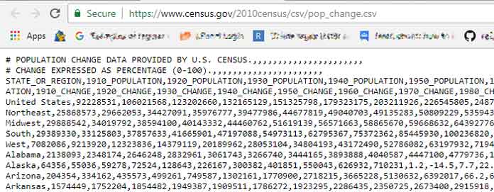
Note: The link is working at the time of writing this post.

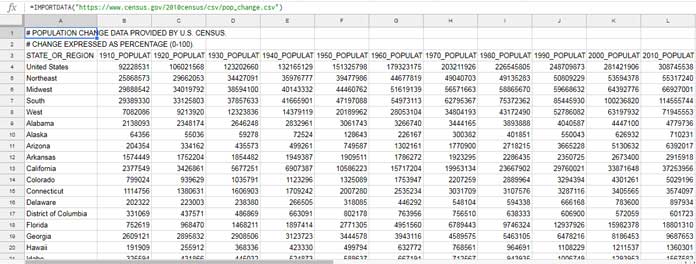
This is the population change data published by the U.S. Census (2010). Let me show you how to import this data in Google Sheets in tabular form.

Open a new Google Sheet and enter this formula in cell A1.

=IMPORTDATA("https://www.census.gov/2010census/csv/pop_change.csv")

This Importdata formula would import the census data in comma delimited format as below in the tabular form.

Apply Data Manipulation Techniques in Imported Data (Query with Importdata Function)

You can use Query with Google Sheets Importdata as below to limit the rows in output.

Limit the Rows Using Query in Importdata Function in Google Sheets

Formula:

=query(IMPORTDATA("https://www.census.gov/2010census/csv/pop_change.csv"),"Select * limit 4")

Change the number four to the total number of rows that you want in the formula output. The above Query and Importdata combination return 4 rows excluding the column label.

Limit the Columns Using Query in Google Sheets Importdata Function

The above formula imports a total of 23 columns. Most of the columns may irrelevant to you.

Here I am limiting the number of columns returned using Query with the Importdata formula.

=query(IMPORTDATA("https://www.census.gov/2010census/csv/pop_change.csv"),"Select Col22,Col23")

Result:

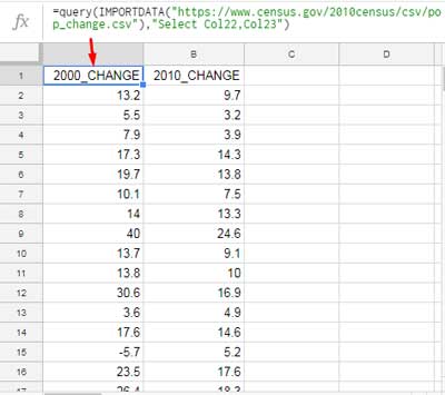
Change the columns in the last part of this Query to return different columns.

Importdata Function with Conditions

The function, by default, doesn’t support conditions in it. Here again, the Query can come in handy.

=query(IMPORTDATA("https://www.census.gov/2010census/csv/pop_change.csv"),"Select * where Col1 = 'California'",3)

This formula only imports the census change data for the region California.

My imported data is not in tabular form. How to make it in tabular form? Read on to find the answer to this question.

Import Txt File Using Importdata Function in Google Sheets

Other than CSV and TSV you can import TXT file using the function Importdata in Google Spreadsheets.

If you use Google Sheets Importdata function to import a text file, the output won’t be in tabular form.

You can, depending on the file, correct that using the Split function.

I don’t have a file to show you an example. So I am providing you a generic formula.

=ArrayFormula(split(QUERY(importdata("your txt file URL.txt"),"Select * offset 5",0)," "))

In this replace the URL with your text file URL that ends with the TXT file extension. Also, change the Offset 5 to the number of rows to offset on the top.

The following simple version will also work well.

=ArrayFormula(IFERROR(split(IMPORTDATA("text file URL.txt"),",")))

In this formula, I have omitted the Query as it’s not a must. We just want to import the data and split the content into columns and rows (tabular form). So this formula will work well in that case.

But please do note that I have put the comma as the delimiter in the just above formula. If your text file is separated by semicolon, then change that accordingly in the formula (see the last part of the formula, after the URL)

That’s all. Any doubt about using the Importdata function in Google Sheets, please let me know.

Related Reading:

1. How to use the IMPORTFEED function in Google Sheets.
2. How to Use IMPORTHTML Function in Google Sheets [Advanced Use]
3. Import Image in Google Sheets using the Image function.
4. Google Sheets IMPORTRANGE Function – Basic to Advanced Use Tips.
5. Align Imported Data with Manually Entered Data in Google Sheets.