In Google Sheets, one can utilize Curly Brackets, also known as Curly Braces, to create Arrays. An array represents a collection of data, typically organized as a table or a range, consisting of rows and columns rather than a single cell.
There are two types of arrays: single-dimensional arrays consist of either a single row or column, while two-dimensional arrays consist of multiple rows and columns.
I understand you likely have many questions about creating arrays in Google Sheets. Through this post, I hope to shed some light on the use of Curly Brackets for creating arrays in Google Sheets.
As a side note, you can also use VSTACK and HSTACK functions to create arrays. For detailed instructions and examples, please refer to the corresponding tutorial in the Google Sheets Function Guide.
Understand the Use of Curly Braces in Google Sheets
Here is an example to explain why Curly Brackets (or VSTACK and HSTACK functions) are necessary to create arrays.
Let’s say you want to reproduce the values in the range A1:B5. If you attempt to use the formula =A1:B5 directly, you’ll encounter a #VALUE! error.
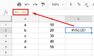
This occurs because while you can refer to a range in a formula simply by mentioning “A1:B5”, you can’t pull or reproduce data from such ranges without using Curly Brackets. That’s why the formula =A1:B5 results in the #VALUE! error.
To resolve this, instead of using =A1:B5, you can use Curly Brackets as shown below to pull the data:
={A1:B5}
=HSTACK(A1:B5) // alternative formula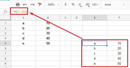
However, is this the only option? No, there are other alternatives such as using ArrayFormula, QUERY, or INDEX functions:
=ArrayFormula(A1:B5)
=QUERY(A1:B5)
=INDEX(A1:B5)
However, the limitation of these alternatives is that you can’t use them to refer to values from distant rows or columns when creating arrays. We’ll explore this further in the examples below.
How to Use Curly Brackets to Create Arrays in Google Sheets
You can combine data from two different ranges either alongside (horizontally) or one under another (vertically) using Curly Brackets.
Horizontal Data Placing Using Curly Brackets
Before we begin, let me ask:
What’s the argument separator in your formulas? Is it a comma or a semicolon? We must know it before utilizing Curly Brackets to combine two ranges horizontally.
For example:
If your argument separator is a comma, you should use the following format:
={A1:B5, E1:F5}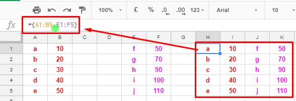
If your argument separator is a semicolon, you should use a backslash instead of a comma, and the formula will be:
={A1:B5 \ E1:F5}It’s important to note that the number of rows in both ranges should be equal, and the ranges in the above formulas satisfy this.
More Examples (My argument separator is a comma):
Single-dimensional array:
={A1, B1, Y1}Two-dimensional array:
={A1:A10, B1:C10, Y1:Y10}Vertical Data Placing Using Curly Brackets
There is no issue with the argument separator in vertical data placement. You should use the semicolon. The only requirement is that the number of columns in both arrays should match.
Example:
={A1:B5; E1:F5}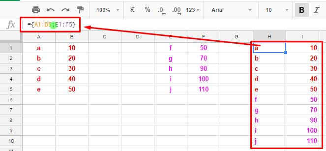
More Examples (My argument separator is a comma):
Single-dimensional array:
={A1; B1; Y1}Two-dimensional array:
={A1:A10; B1:C10; Y1:Y10}Data From Two Different Sheets in the Same File
Now, let me explain how to use Curly Braces to create an array from different sheets within the same file.
In this case, you simply include the sheet name along with the cell range.
Example 1: Horizontal
={Sheet1!A1:B5, Sheet2!A1:B5}Note: In this formula, if your argument separator is a semicolon, use a backslash (\) instead of a comma.
Example 2: Vertical
={Sheet1!A1:B5; Sheet2!A1:B5}Control the #REF Error Due to Infinite Rows in Combined Arrays
In the above examples, we have used closed arrays such as A1:B5 and E1:F5. Can we replace these closed arrays with open arrays such as A1:B and E1:F?
In most cases, replacing closed arrays with open arrays will result in a #REF error. However, you can avoid this issue by using the QUERY function in Google Sheets. Here is an example:
Consider the content in “Sheet1” and “Sheet2”. You can combine them in “Sheet3” using a Query formula as follows:
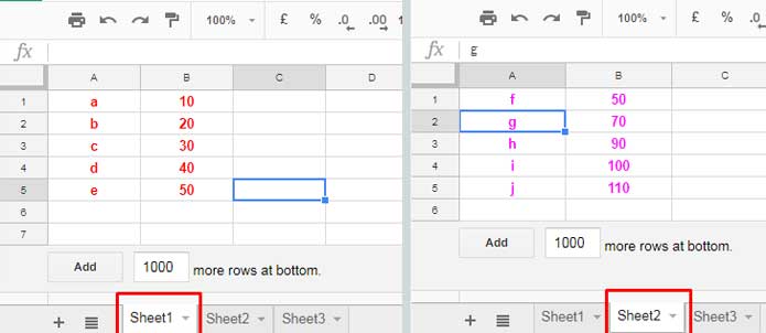
To combine and pull data vertically, keeping the range open (with the number of columns equal), you can use:
=QUERY(
  {Sheet1!A1:B; Sheet2!A1:B},
  "Select * where Col1 is not null"
)
For horizontal combination (with the number of rows equal), you can use:
={
   QUERY({Sheet1!A1:B}, "Select * where Col1 is not null"),
   QUERY({Sheet2!A1:B}, "Select * where Col1 is not null")
}
I have applied the same technique to create data consolidation in Google Docs Spreadsheets.
Creating Arrays Using Curly Brackets and Their Real-life Applications
The VLOOKUP function is an excellent tool to demonstrate the use of arrays created with Curly Braces. Here are two examples:
Example 1:
Assume we have a table in the range A1:F6 with the following data:
| ID | Name | Age | Gender | Height | Weight |
| 1 | Catherine | 26 | M | 180 | 77 |
| 2 | Jane | 31 | F | 165 | 61 |
| 3 | Joshua | 38 | M | 175 | 79 |
| 4 | Emily | 27 | F | 170 | 66 |
| 5 | Michael | 28 | F | 160 | 55 |
The following formula will search for ID 4 in column A and return Name, Age, Gender, Height, and Weight:
=ArrayFormula(VLOOKUP(4, A1:F6, {2, 3, 4, 5, 6}, FALSE))Syntax: VLOOKUP(search_key, range, index, [is_sorted])
Since we want to return multiple values, we have used the ArrayFormula function with this VLOOKUP.
In the ‘index’ parameter, we have used Curly Brackets to create a single-dimensional horizontal array representing columns 2 to 6.
Related: Multiple Values Using Vlookup in Google Sheets
Example 2:
VLOOKUP is capable of searching only the first column of the range. If you want to search for a name and return his ID, you can create an array with the name in the first column and the ID in the second column:
=VLOOKUP("Jane", {B1:B, A1:A}, 2, FALSE)Conclusion
We have seen how to create arrays using Curly Brackets from data in the same sheet and across multiple sheets.
I suggest considering the use of VSTACK and HSTACK functions for creating arrays, as they accommodate situations where the number of rows (for horizontal array creation) or the number of columns (for vertical array creation) differs in the arrays being combined.
Furthermore, you need not worry about the separator used, as you only need to follow the argument separator specified in your formula, which will be either a comma or semicolon.


Please help Why is this formula not working?
=QUERY({'Duplicates 2'!$A$2:$P$1000;'Duplicates 3'!$A$2:$P$1000}, "SELECT A,B,C,D WHERE P = 1 ORDER BY E ASC")Hi, Nicole,
Use Col1, Col2,… instead of A,B,…
While I am using
={Sheet1!A1:B5; Sheet2!A1:B5}, it is just showing me an error.Can you please help me with this? It will be helpful.
Hi, Sonali,
Your formula seems correct to me.
There may be several reasons for an error.
If you share a sample/copy of your sheet by leaving the URL below, I may be able to help.
I am using this in the SharePoint excel sheet. I can’t share the URL. Can you suggest in any other way? It will be really helpful.
Can an array formula use a range in a separate file? (Not a separate sheet).
Hi, Colin,
Yes! You can import the data and use it.
This may help – How to Use Query with Importrange in Google Sheets.
Thank you very much, your presentation is clear and precise, it has helped me a lot.
Hi, thanks for including the statement “in some countries like the UK, you may need to use backslash instead of the comma.” I spent days trying to figure out why the formula (using comma) didn’t work in my sheet. It finally works now. Phew. I owe you Prasanth.
Is it possible to join two arrays horizontally? I have several formulas like:
=ArrayFormula(transpose("some text - "&INDIRECT(someDynamicRange)))which all take data from dynamically defined range and create column names. What I would like to achieve is to “add” these formulas in order to create all the columns that I need. The syntax like:
{{transpose("some text - "&INDIRECT(someDynamicRange)}\{transpose("some other text - "&INDIRECT(someOtherDynamicRange)}}interestingly returns just the second item from the first array and an error: An array value could not be found.
Thank you for your reply.
Andrej
Hi, Andrej Mocan,
The number of rows in each formula output must match.
Best,
I was always confused about the use of curly brackets, comma, semi-colon. Now with the article. I come to know. Thanks a ton. Prasanth.