


")


")

")
")
 in Excel & Google Sheets")


You can use an array formula in Google Sheets to calculate subtotals up to the first blank cell and after each subsequent blank cell. Furthermore, you can control where to place the subtotals – either corresponding to the blank cell or one row above it, i.e., in the last row of each group separated by blank cells.
The benefit of the array formula is that you do not need to adjust it each time you add more data, or insert or delete rows.
Example: Calculate Subtotals Up to the First Blank Cell and Insert Them in Google Sheets
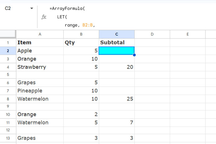
Assume you have values in B2:B, separated by blank rows. The blank rows may occur at specific intervals, such as every 7 rows, or at irregular intervals. You want to calculate the subtotals up to the first blank cell and after each subsequent blank cell.
In that case, use the following formula in cell C2:
=ArrayFormula(
LET(
range, B2:B,
_rows, IF(INDIRECT("B2:B"&XLOOKUP(TRUE, range<>"", ROW(range), ,0, -1)+1)="", ROW(range),),
_rowsE, {ROW(B2); TOCOL(_rows, 1)},
seq, SEQUENCE(ROWS(_rowsE)),
total, MAP(_rowsE, seq, LAMBDA(x, y, SUMIF(ISBETWEEN(ROW(range), x, CHOOSEROWS(_rowsE, y+1), TRUE, FALSE), TRUE, range))),
data, HSTACK(TOCOL(_rows, 1), total),
IFNA(VLOOKUP(ROW(range)+1, data, 2, FALSE))
)
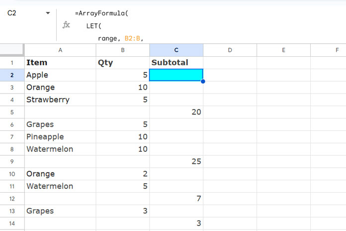
)This formula will place the subtotals in the bottom row of each section separated by blank cells.
If you want the subtotals next to each blank cell, simply remove +1 within the VLOOKUP function.
How Do I Adapt This Formula to My Data Range?
The formula is designed for the range B2:B. To adapt it to your data range, update the following references:
- For example, if your data range is
E5:E, insert the formula inF5, assumingF5:Fis empty. - Replace all occurrences of
B2:Bwith your data range (e.g.,E5:E). - Replace
B2with the first cell in your range (e.g.,E5).
Formula Explanation
_rows:
IF(INDIRECT("B2:B"&XLOOKUP(TRUE, range<>"", ROW(range), ,0, -1)+1)="", ROW(range),)This part identifies the row numbers corresponding to blank cells in the column to subtotal. It also includes the row number below the last non-empty cell to ensure the formula covers all data groups.
_rowsE:
{ROW(B2); TOCOL(_rows, 1)}This step removes empty cells from _rows and adds the row number of the first cell in the range to the top of the array.
seq:
SEQUENCE(ROWS(_rowsE))Generates sequence numbers corresponding to _rowsE.
total:
MAP(_rowsE, seq, LAMBDA(x, y, SUMIF(ISBETWEEN(ROW(range), x, CHOOSEROWS(_rowsE, y+1), TRUE, FALSE), TRUE, range)))Uses the MAP function to iterate through _rowsE (row numbers of blank cells and the first row) and seq (sequence numbers). The lambda function sums the values in the range between each pair of rows.
data:
HSTACK(TOCOL(_rows,1), total)Creates a two-column array where the first column contains row numbers corresponding to blank cells and the second column contains the corresponding subtotals.
Final Formula Expression:
IFNA(VLOOKUP(ROW(range)+1, data, 2, FALSE))Uses VLOOKUP to find the subtotal for each row in the range and display it in the appropriate position.
Resources
- Reset Running Total at Blank Rows in Google Sheets
- Group and Sum Data Separated by Blank Rows in Google Sheets
- Grouping and Subtotal in Google Sheets and Excel
- Insert Subtotal Rows in a Google Sheets Query Table
- AT_EACH_CHANGE Named Functions in Google Sheets
- Formula to Insert Group Total Rows in Google Sheets
Sorry I didn’t add function number that was my mistake. I forget that. Thanks for these tips and tricks 🙂
Welcome!
Hi, how can we do this with subtotal function? I changed it but it didn’t work. Why I need this because I use the filter in my sheet. I want to sum filtered numbers. I read your this post too: https://infoinspired.com/google-docs/how-to-omit-hidden-or-filtered-out-values-in-sum-google-doc-spreadsheet/