Google Sheets offers three powerful functions for advanced sorting capabilities: SORT, SORTN, and QUERY. These functions allow you to sort data in Google Sheets efficiently. Additionally, there’s the SORT menu option for basic sorting. This tutorial explains how to sort data in Google Sheets using these functions, including different formulas and sort orders.

Sort Orders: Ascending and Descending

In Google Sheets, you can sort structured tables, ranges, single columns, or distant columns in ascending (A-Z) or descending (Z-A) order using the SORT, QUERY, or SORTN functions.

• Ascending Order: Lowest values appear at the top of the column.
• Descending Order: Highest values appear at the top of the column.

Empty cells are treated differently depending on the function used:

• SORT and SORTN place empty rows at the bottom, regardless of sort order.
• QUERY places empty rows at the top in ascending order and at the bottom in descending order. However, it has an option to filter out empty rows.
• Additionally, QUERY allows you to keep the header row at the top, whereas SORT and SORTN move it based on the sorting order. When using SORT or SORTN, exclude the header row to prevent it from being sorted.

Sorting Data in a Range in Google Sheets

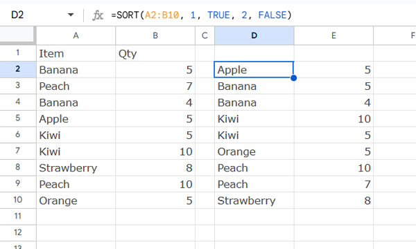
Let’s say you have fruit names in Column A and their quantities in Column B within the range A1:B10 , with headers in the first row. Some fruits are repeated.

Goal: Sort the range by fruit names in ascending order. If fruits are repeated, sort by quantity in descending order.

Using SORT:

=SORT(A2:B10, 1, TRUE, 2, FALSE)

• A2:B10: Range to sort.
• 1: First sort column (fruit names).
• TRUE: Sort in ascending order.
• 2: Second sort column (quantities).
• FALSE: Sort in descending order.

Ref.: Google Sheets SORT Function: Usage and Examples

Using SORTN:

=SORTN(A2:B10, 9, 0, 1, TRUE, 2, FALSE)

• 9 Specifies the number of rows to return after sorting.
• 0 Represents the display_ties_mode for standard sorting (similar to SORT). Other modes can handle duplicates differently.
• 1 and 2 are the sort columns.
• TRUE and FALSE set the sort orders.

When compared to the SORT function, this formula includes two additional arguments: the number of rows to return and the display ties mode.

Ref.: How to Use the SORTN Function in Google Sheets

Using QUERY:

=QUERY(A2:B10, "WHERE Col1 IS NOT NULL ORDER BY Col1 ASC, Col2 DESC", 0)

• Col1 (first column) is sorted in ASC (ascending) order.
• Col2 (second column) is sorted in DESC (descending) order.
• The WHERE Col1 IS NOT NULL condition filters out empty rows.

To retain the header row, use:

=QUERY(A1:B10, "WHERE Col1 IS NOT NULL ORDER BY Col1 ASC, Col2 DESC", 1)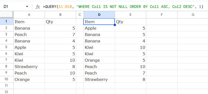

Ref.: Learn Google Sheets QUERY Function: Step-by-Step Guide

Sorting Data in Two Distant Columns

If your data is in distant columns (e.g., A2:A10 contains fruit names and C2:C10 contains quantities), use HSTACK to combine them horizontally before sorting.

Using SORT:

=SORT(HSTACK(A2:A10, C2:C10), 1, TRUE, 2, FALSE)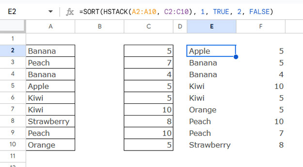

SORTN and QUERY Alternatives:

=SORTN(HSTACK(A2:A10, C2:C10), 9, 0, 1, TRUE, 2, FALSE)

=QUERY(HSTACK(A2:A10, C2:C10), "WHERE Col1 IS NOT NULL ORDER BY Col1 ASC, Col2 DESC", 0)

Sorting Data Based on a Column Outside the Sort Range

To sort a range based on a column outside the sort range (e.g., sorting weekday names in A2:A8 based on weekday numbers in C2:C8), use:

=SORT(A2:A8, C2:C8, TRUE)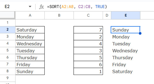

Here is the SORTN Alternative:

=SORTN(A2:A8, 7, 0, C2:C8, TRUE)

When using QUERY, append the sort column horizontally and use the SELECT clause to exclude it from the final output.

=QUERY(HSTACK(A2:A8, C2:C8), "SELECT Col1 WHERE Col1 IS NOT NULL ORDER BY Col2 ASC", 0)

Sorting Data Using Structured Table References

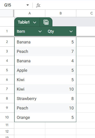
A major benefit of structured table references is that they adjust dynamically when the table expands. Assume your table is named “Table1” with two columns: Item and Qty.

Formulas for Sorting Using Structured Table References:

=SORT(Table1, 1, TRUE, 2, FALSE)

=SORTN(Table1, 9, 0, 1, TRUE, 2, FALSE)

=QUERY(Table1, "WHERE Col1 IS NOT NULL ORDER BY Col1 ASC, Col2 DESC", 0)

To retain headers:

=QUERY(Table1[#ALL], "WHERE Col1 IS NOT NULL ORDER BY Col1 ASC, Col2 DESC", 1)

Is There a Function That Does the Opposite of Sorting?

While there’s no direct function to reverse sorting, you can randomize data using SORT and RANDARRAY:

=SORT(A2:B10, RANDARRAY(ROWS(A2:B10)), TRUE)

To keep the randomized order, copy the result and paste as values:

• Edit > Copy > Edit > Paste Special > Values Only

Google Sheets also has a Data > Randomize range menu option for this purpose.

Conclusion

This tutorial covered how to sort data in Google Sheets using SORT, QUERY, and SORTN, along with methods for handling structured tables and sorting non-adjacent columns. Mastering these functions will help you efficiently organize and analyze your data.

Resources

Explore these additional guides to master sorting in Google Sheets:

1. Sort by Custom Order in Google Sheets
2. Sort by Month Name in Google Sheets
3. Sort Horizontally (Left to Right) in Google Sheets
4. Custom Sort Order in Google Sheets Query
5. Sort Alphanumeric Values in Google Sheets
6. Sort by Date of Birth in Google Sheets
7. Sort by Number of Occurrences in Google Sheets
8. Sort Merged Cells in Google Sheets
9. Row-Wise Sorting in a 2D Array
10. Custom Sort by Partial Match in Google Sheets