Is it possible to filter rows based on row numbers in Google Sheets? Yes! You can use row numbers as Filter criteria in Google Sheets.

To filter rows based on given row numbers, you can use the function Filter. That means, in the Filter, the criteria/conditions will be row numbers.

Actually, the formula, using row numbers as the criteria in the Filter function, is very easy to code. Before that, we must understand the real-life use of such filtering.

Row Numbers as Filter Criteria in Real Life Use in Google Sheets

For our tutorial purpose, I am going to import some data into one of my Google Sheets files from the below source page on Wikipedia. It’s the happiness index of the world countries – World Happiness Report – Wiki.

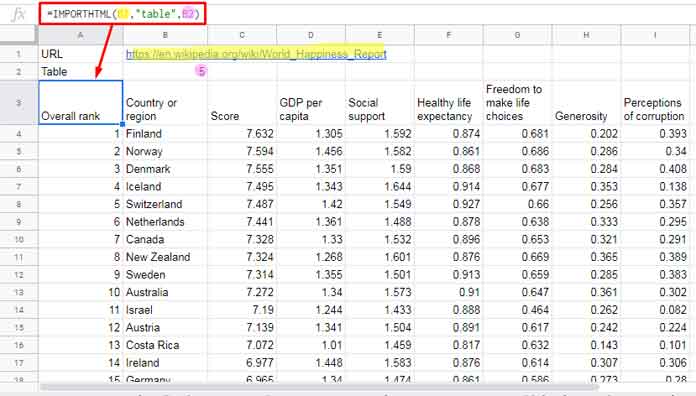
By using the following IMPORTHTML formula, you can get that happiness index data in Google Sheets.

=IMPORTHTML(B1,"table",B2)

I have keyed this formula in cell A3. Cell B1 contains the URL of the above Wiki page and cell B2 contains the table number.

The formula will import the whole table that contains around 150 rows into my Google Sheets file. Here are the formula and the first few rows.

Now we have a sample dataset to test the said type of Filter.

Are you familiar with the Match function in Sheets? If not, please check my guide – How to Use Match Function in Google Sheets.

The Match function in Sheets can search a key and return relative position of that key/item in the dataset. See the below example.

Assume you want to find the relative position of the value “Australia” in the range B4:B in our above sample data. For that, you can use this Match formula.

=match("Australia",B4:B,0)

This formula would return 10, that’s the relative position of the key “Australia” in the range B4:B.

If you start counting from B4, you can find the key “Australia” in the 10th position.

Normally we use such relative position in Index function to offset rows. You can check my Index-Match tutorial for that usage. Here you will get one example.

Offsetting Relative Position Using Index in Google Sheets

Must Check: Google Sheets Function Guide [Quickly Learn All Popular Functions].

See the image above for the array/range used in this Index-match formula.

=index(A4:I,match("Australia",B4:B,0),0)

This formula is equal to;

=index(A4:I,10,0)

This will return the 10th row from the provided range. What if when there are multiple keys in Match and multiple relative positions?

Offsetting Nonconsecutive Relative Position in Google Sheets

Then the Index won’t come in handy as the function can’t offset nonconsecutive relative positions.

In such a case, you can convert that relative positions of the keys into corresponding row numbers. Then use that row numbers to filter rows by row numbers.

That’s the purpose of using row numbers as Filter criteria in real life in Google Sheets. I am going to explain that usage here in this tutorial.

Converting Relative Position to Row Number in Google Sheets

Relative Position to Row Number – One Search Key

First, check the range used in the Match formula above. It’s B4:B. That means the range starts from the fourth row. So you can add #3 to the Match output, which is 10, to get the actual row number from that relative position.

Instead of adding 3 make it dynamic. Here is the formula that converts the relative position to the corresponding row number in Google Sheets.

Formula # 1:

=match("Australia",B4:B,0)+row(B3)

This formula would return 13 as the row number. The Row formula returns #3.

What about multiple keys in the Match?

Relative Positions to Row Numbers – Multiple Search Key

Take a look at this Match formula that uses two search keys.

Formula # 2:

=ArrayFormula(match({"Australia","Germany"},B4:B,0)+row(B3))

This formula would return the row numbers 13 and 18. The search key “Australia” is in the 13th row and the key “Germany” is in the 18th row.

You have learned how to convert relative positions to corresponding row numbers. Let me show you how to use these row numbers to extract those rows in Google Sheets.

How to Use Row Numbers as Filter Criteria in Google Sheets

First, let me explain to you how to use row numbers as Filter criteria in Google Sheets. Then we can replace that row numbers with the Match formula. That means we will use dynamic row numbers in filtering.

Row Number as the Criterion in Google Sheets Filter Function

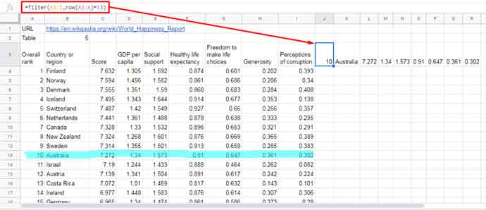
I have the following Filter formula in cell J4 that uses the number 13 (row number) as the criterion.

=filter(A3:I,row(A3:A)=13)

The formula extracts the highlighted row, which is the 13th row.

To feed dynamic row numbers replace row(A3:A)=13 in the formula with the above Match Formula # 1. Here is that.

=filter(A3:I,row(A3:A)=match("Australia",B4:B,0)+row(B3))

Row Numbers as the Criteria in the Filter Function in Google Sheets

How to use multiple-row numbers as the criteria in Filter in Google Sheets?

In one of my earlier post, I have elaborated on how to use multiple conditions in the same column (OR condition) in Filter – How to Use AND, OR with Google Sheets Filter Function.

The following formula is in line with the tips detailed in that tutorial.

=filter(A3:I,(row(A3:A)=13)+(row(A3:A)=18))

This Google Sheets formula will filter the rows 13 and 18. How to make it dynamic by replacing two of the Row formulas with our Match Formula # 2?

That’s a little tricky and somewhat complicated. But don’t worry! I will try to explain that.

Here I am including step by step instructions.

Step 1:

We must first convert the Formula # 2 to output as below.

^13$|^18$

How? To get this use Textjoin function with the Match Formula # 2.

=ArrayFormula(textjoin("|",true,"^"&(match({"Australia","Germany"},B4:B,0)+row(B3)&"$")))

Step 2:

Use the above formula as the regular_expression in Regexmatch. I mean replace "^13$|^18$" in the following formula with the just above formula.

=ArrayFormula(regexmatch(row(A4:A)&"","^13$|^18$"))

So the formula will be;

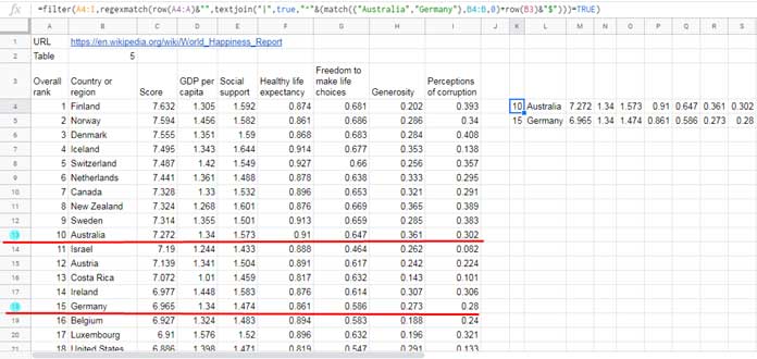
=ArrayFormula(regexmatch(row(A4:A)&"",textjoin("|",true,"^"&(match({"Australia","Germany"},B4:B,0)+row(B3)&"$"))))

To test it, just enter it in cell J4. You can see that the formula returns TRUE against row numbers 13 and 18. In all the other rows, it returns FALSE.

Now we want a formula like this to return the rows containing TRUE.

Generic Formula:

=filter(A4:I,regexmatch_formula=TRUE)

Replace regexmatch_formula with the formula above and that final formula will be as below.

=filter(A4:I,regexmatch(row(A4:A)&"",textjoin("|",true,"^"&(match({"Australia","Germany"},B4:B,0)+row(B3)&"$")))=TRUE)

This way you can use row numbers as Filter criteria in Google Sheets.

Related Reading: Filter Out Matching Keywords in Google Sheets – Partial or Full Match.