The RECEIVED function in Google Sheets is a financial function used to calculate the amount received at maturity for investments in fixed-income securities such as bonds, asset-backed securities (ABS), and similar instruments.
You don’t need to be a financial analyst to calculate the return on a bond you’ve purchased! You can easily use Google Sheets for this—just type https://sheets.new/ in your browser’s address bar to get started.
By entering input values like the settlement date, maturity date, and discount rate, you can calculate the bond’s maturity amount using the RECEIVED function in Google Sheets.
To make things easier, I’ll explain the syntax and arguments of the RECEIVED function in detail.
Google Sheets RECEIVED Function – Syntax and Arguments
Syntax
RECEIVED(settlement, maturity, investment, discount, [day_count_convention])Arguments
There are five arguments in the RECEIVED function—four required and one optional:
- settlement – The settlement date of the security, i.e., the date after issuance when the bond is delivered to the buyer.
Example: If a 6-year bond is issued on January 1, 2014, and purchased three months later, the settlement date would be April 1, 2014. - maturity – The maturity date of the security, when it can be redeemed at its face (or par) value.
Continuing the example above, the maturity date would be January 1, 2020. - investment – The amount invested in the security.
- discount – The discount rate or rate of return.
- day_count_convention (optional) – Determines how days are counted for interest calculation. The default is
0. See the table below for more details.
Day Count Convention Table
| day_count_convention | Description |
|---|---|
| 0 or omitted | US (NASD) 30/360 |
| 1 | Actual/Actual |
| 2 | Actual/360 |
| 3 | Actual/365 |
| 4 | European 30/360 |
RECEIVED Function Example in Google Sheets
Let’s walk through an example of how to use the RECEIVED function in Google Sheets to calculate the maturity amount of a bond.
Assume:
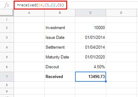
- Initial investment: $10,000
- Discount rate: 4.5%
- Settlement date: April 1, 2014
- Maturity date: January 1, 2020
Note: In simple terms, a bond is an instrument of indebtedness—it represents a loan made by a bondholder to an issuer.
Formula:
=RECEIVED(C4, C5, C2, C6)In this example using the RECEIVED function in Google Sheets, I’ve omitted the optional day_count_convention argument. By default, it’s treated as 0, which means the US (NASD) 30/360 basis is used (refer to the table above).
Example with Hardcoded Arguments
When entering dates directly in the formula, it’s best to use the DATE function to prevent formatting errors. Use the format DATE(year, month, day).
=RECEIVED(DATE(2014, 4, 1), DATE(2020, 1, 1), 10000, 4.5%)Possible Errors When Using the RECEIVED Function
The two common errors you may encounter while using the RECEIVED function in Google Sheets are #VALUE! and #NUM!.
VALUE! Error – Causes
- Settlement or maturity dates are in invalid formats.
NUM! Error – Causes
- Investment amount or discount rate is missing.
- Either investment or discount rate is less than or equal to zero.
- An invalid
day_count_conventionis entered (should be omitted or 0–4). - Settlement date is equal to or later than the maturity date.
That’s it! Now you know how to confidently use the RECEIVED function in Google Sheets to calculate bond maturity values. Give it a try with your own data and explore more financial functions in Sheets!


