


")


")

")
")
 in Excel & Google Sheets")


In Google Sheets, the QUERY function is the perfect tool to summarize data, regardless of whether the data type is text, numbers, or dates. Without a doubt, QUERY is the best function to create daily, weekly, monthly, quarterly, and yearly summary reports in Google Sheets.
Daily transactions are a crucial part of many businesses, especially in sales. No matter what type of business you run, you likely have data to record daily—whether it’s sales, purchases, or cash transactions. Even bloggers have their daily data to track, such as site traffic, page impressions, CTR, and more.
In such cases, you might want to create a summary of your daily transactions, traffic, or any other activity you record. Below, I’ll show you how to create daily, weekly, monthly, quarterly, and yearly summary reports in Google Sheets using the QUERY function.
You can use my formulas directly by adjusting your sales/purchase report columns to match my format. I’ve included a sample sheet with formulas and demo data at the end of this tutorial.
Including all the daily, weekly, monthly, quarterly, and yearly summary reports in one tutorial serves a purpose. You can convert daily reports into other types (except weekly) by simply modifying the scalar function used. I hope you’ll appreciate how I’ve laid out the formulas below.
Query Scalar Functions to Create Daily, Weekly, Monthly, Quarterly, and Yearly Summary Reports
In the QUERY function, you can use the following scalar functions to create summary reports based on a date column (a column containing transaction dates):
month(): Returns the month value from a date or datetime value. It’s zero-based, meaning month numbers range from 0 to 11, where 0 represents January and 11 represents December. To get standard month numbers (1–12), usemonth()+1.quarter(): Returns the quarter from a date or datetime (timestamp) value.year(): Returns the year value from a date or datetime (timestamp) value.
For weekly reports, there’s no specific scalar function in QUERY. Instead, we’ll use a native Google Sheets function to convert dates into weeks and use that column for summarization.
Let’s use these QUERY scalar functions and native Sheets functions to create daily, weekly, monthly, quarterly, and yearly summary reports in Google Sheets.
Sample Data
For all examples, we’ll use the following basic data to easily check the results:
| Date | Product | Qty |
| 08/01/2025 | Red Sand | 150 |
| 08/01/2025 | Red Sand | 150 |
| 16/01/2025 | Black Sand | 80 |
| 07/02/2025 | 3/16 Aggregate | 280 |
The sample data is in columns A1:C , with sales dates, products, and sales quantities (in tonnage).
1. Query to Create Daily Summary Reports in Google Sheets
Suitable when you have multiple transactions in a day:
You might be surprised to learn that you can use the QUERY function on this sample data to create five different types of daily summary reports.
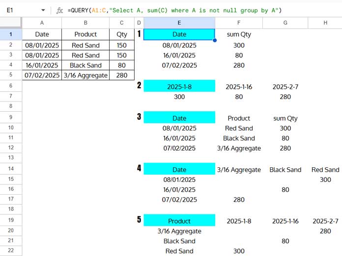
1. Grouped by Date:
=QUERY(A1:C,"Select A, sum(C) where A is not null group by A")2. Pivoted by Date:
=QUERY(A1:C,"Select sum(C) where A is not null pivot A")3. Grouped by Date and Product:
=QUERY(A1:C,"Select A,B, sum(C) where A is not null group by A,B")4. Grouped by Date, Pivoted by Product:
=QUERY(A1:C,"Select A, sum(C) where A is not null group by A pivot B")5. Grouped by Product, Pivoted by Date:
=QUERY(A1:C,"Select B, sum(C) where A is not null group by B pivot A")Out of these five QUERY formulas, choose the one that suits your needs for creating a daily summary report. Once you understand these formulas, converting them to create monthly, quarterly, and yearly summary reports becomes straightforward.
Tip: In the above formulas, I used the SUM() aggregation function. You can replace it with AVG(), MIN(), MAX(), or COUNT() depending on your reporting needs.
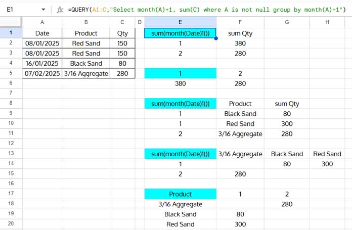
2. Query to Create Monthly Summary Reports in Google Sheets
Suitable when you have data spanning multiple months in a year and multiple transactions per month:
To transform the daily summary report into a monthly summary report, replace A with month(A)+1 in the SELECT, GROUP BY, and PIVOT clauses. Here are the updated formulas:
=QUERY(A1:C,"Select month(A)+1, sum(C) where A is not null group by month(A)+1")=QUERY(A1:C, "Select sum(C) where A is not null pivot month(A)+1")=QUERY(A1:C, "Select month(A)+1, B, sum(C) where A is not null group by month(A)+1, B")=QUERY(A1:C, "Select month(A)+1, sum(C) where A is not null group by month(A)+1 pivot B")=QUERY(A1:C,"Select B, sum(C) where A is not null group by B pivot month(A)+1")
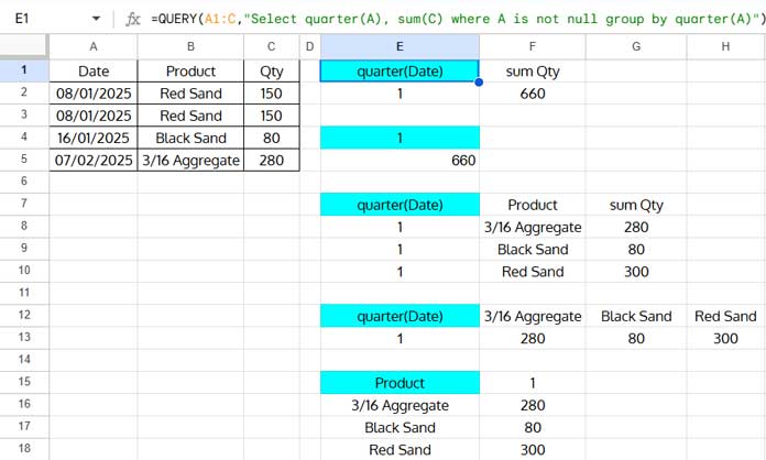
3. Query to Create Quarterly Summary Reports in Google Sheets
Suitable when you have data spanning multiple quarters in a year and multiple transactions per quarter:
For quarterly reports, use the quarter() function instead of month(). Here are the formulas:
=QUERY(A1:C,"Select quarter(A), sum(C) where A is not null group by quarter(A)")=QUERY(A1:C, "Select sum(C) where A is not null pivot quarter(A)")=QUERY(A1:C, "Select quarter(A), B, sum(C) where A is not null group by quarter(A), B")=QUERY(A1:C, "Select quarter(A), sum(C) where A is not null group by quarter(A) pivot B")=QUERY(A1:C,"Select B, sum(C) where A is not null group by B pivot quarter(A)")
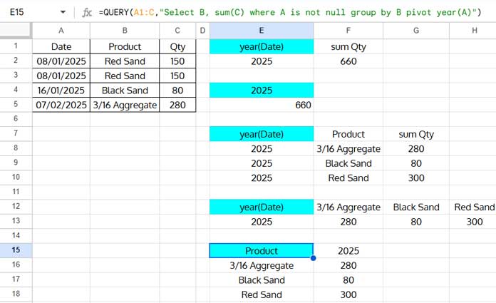
4. Query to Create Yearly Summary Reports in Google Sheets
Suitable when you have data spanning multiple years:
To create yearly summary reports, use the year() function in the SELECT, GROUP BY, and PIVOT clauses:
=QUERY(A1:C,"Select year(A), sum(C) where A is not null group by year(A)")=QUERY(A1:C, "Select sum(C) where A is not null pivot year(A)")=QUERY(A1:C, "Select year(A), B, sum(C) where A is not null group by year(A), B")=QUERY(A1:C, "Select year(A), sum(C) where A is not null group by year(A) pivot B")=QUERY(A1:C,"Select B, sum(C) where A is not null group by B pivot year(A)")
5. Query to Create Weekly Summary Reports in Google Sheets
Suitable when you have data spanning multiple weeks in a year:
Creating weekly reports is slightly more complex. To simplify, we’ll use a helper column.
In cell D1, enter the following formula to return week numbers corresponding to the dates in column A:
=ArrayFormula(VSTACK("Week #", WEEKNUM(A2:A, 2)*(A2:A<>"")))This returns Monday–Sunday week numbers. For Sunday–Saturday weeks, replace 2 with 1 in the WEEKNUM function.
Now, use the QUERY formulas for daily reports with two changes:
- Select the data range
A1:Dinstead ofA1:Cto include the helper column. - Replace column
Ain the SELECT, GROUP BY, and PIVOT clauses with columnD.
Here are the updated formulas:
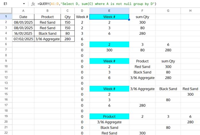
1. Grouped by Week:
=QUERY(A1:D,"Select D, sum(C) where A is not null group by D")2. Pivoted by Week:
=QUERY(A1:D, "Select sum(C) where A is not null pivot D")3. Grouped by Week and Product:
=QUERY(A1:D,"Select D, B, sum(C) where A is not null group by D,B")4. Grouped by Week, Pivoted by Product:
=QUERY(A1:D,"Select D, sum(C) where A is not null group by D pivot B")5. Grouped by Product, Pivoted by Week:
=QUERY(A1:D,"Select B, sum(C) where A is not null group by B pivot D")Conclusion
The formulas above are the simplest way to create daily, weekly, monthly, quarterly, and yearly summary reports in Google Sheets.
You may want to customize these reports further—for example, displaying month names instead of numbers, showing week start and end dates instead of week numbers, or summarizing by month and year.
For more advanced techniques, explore the resources below or search this site.
Resources
- How to Group Data by Month and Year in Google Sheets
- Google Sheets: Using SUMIF to Sum by Month and Year
- Group Dates in Pivot Table in Google Sheets (Month, Quarter, and Year)
- Creating Month-Wise Summary in Google Sheets (Query Formula)
- Sum Data by Month (Not Year) in Google Sheets with SUMIF
- Google Sheets Query: Convert Month Number to Month Name
- Creating a Weekly Summary Report in Google Sheets
- How to Group by Week in Pivot Table in Google Sheets
- How to Sum by Week of the Month in Google Sheets
- How to Sum Values by the Current Week in Google Sheets
- Query to Calculate Hours Worked Week-Wise in Google Sheets
- Sum Current Work Week Range with QUERY in Google Sheets
- SUMIF to Sum by Current Work Week in Google Sheets
- Summarize Data by Week Start and End Dates in Google Sheets
- How to Group Dates by Quarter in Google Sheets
Can I group by year, month, week day and say an elapsed time duration worked on.
And can I do the same thing by adding in the Project column too?
Hi, David,
Before trying, I wish to see a sample of your data (mockup) and your expected output.
Can you share one sheet via your reply below?
Hi Prashanth,
Your content is awesome and a lifesaver for me at the moment!
Quick question, though, on this.
Is it possible to query data across multiple years and have it count by year and quarter?
I’ve used the following to get the entries per year, and it’s worked:
=query(Sheet1!A:J,"select year(A), Count(A) Group By year(A)")And this gives me per quarter:
=query(Sheet1!$A:$J,"select Quarter(A), Count(A) Group By quarter(A)")Ideally, I’d like by year and quarter.
Many thanks in advance for your help,
Ian
Hi, Ian Leonard,
This may help.
=query(Sheet1!$A:$J,"select year(A),quarter(A),Count(A) where A is not null Group By year(A),quarter(A)")
Please include the WHERE clause in your formulas above to skip blank rows.
This is really helpful, thanks! How do you basically do this whilst maintaining a row for every day even if there isn’t a value for a day?
Hi, Penny,
I can hopefully help you if you can provide (share URL) a mockup sheet.
What if I want to sum the monthly mileage for a specific individual by day of the month?
I have a mileage log that lists the date, who the mileage is for, and how many miles were driven. There are multiple entries for each individual each day.
I want it to add all mileage (column I) of RK (one of the people in Column C) and have total ‘RK’ miles reported by day of the month.
I’ve been trying this:
=QUERY(A8:I100," select A where C='RK',sum(I) group by A")but it gives an error. Can’t seem to find a fix.Hi, Cindy,
The Query formula syntax is not correct. Please see my Query Clause order guide.
So, you should rewrite the formula as below.
=QUERY(A8:I100,"Select A, sum(I) where C='RK' group by A")Also, you should understand the changes in formulas as per regional settings.
The formulas in my tutorials are as per the LOCALE set to the UK in the File menu Spreadsheet settings.