Google Sheets’ COUNTIFS function can return the count of an array or range based on multiple conditions. But what if one of those conditions is ‘not blank’? This quick tutorial will show you how to use ‘not blank’ as a condition in the COUNTIFS function in Google Sheets.
In this tutorial, I’ll focus on two key scenarios:
- Using ‘not blank’ as a criterion in one column while applying another criterion from a different column.
- Applying ‘not blank’ as a condition in one column and an additional condition from the same column.
This tutorial is centered on these two points, and I’ll keep it concise and straightforward. Let’s dive in!
Using ‘Not Blank’ as a Criterion in Conditional Counting
Use the <> operator to specify ‘not blank’ in a COUNTIFS (conditional count). The following COUNTIFS formula will count all the non-blank cells in the range A1:A10:
=COUNTIFS(A1:A10, "<>")However, you don’t need to use COUNTIFS for this. The COUNTIF function can achieve the same result:
=COUNTIF(A1:A10, "<>")The true purpose of COUNTIFS is to count based on multiple criteria. Let’s explore how to use ‘not blank’ as one of the conditions in COUNTIFS in Google Sheets.
COUNTIFS with ‘<>’ in One Column and Another Condition in a Different Column
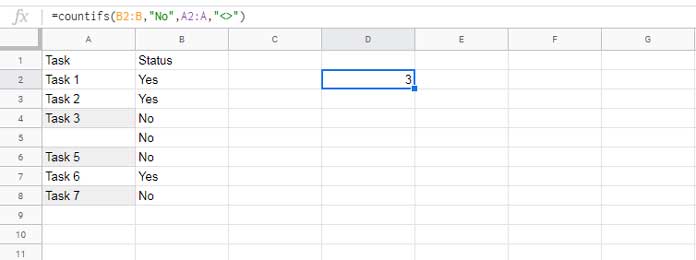
Let’s apply the COUNTIFS formula to the sample dataset below, which contains task names in column A and their status in column B. This will make it easier for me to explain the conditions.
=COUNTIFS(B2:B, "No", A2:A, "<>")
Explanation:
The purpose of this formula is to count all the unfinished tasks in column A.
The “Status” (column B) is equal to “No,” meaning the task is not finished. However, some task names in column A are still blank. I don’t want to count every “No” in column B—only those where the corresponding cells in column A are filled. That’s what the above COUNTIFS formula does.
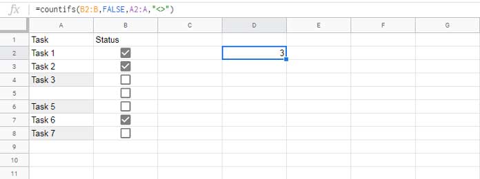
If you are using tick boxes instead of “Yes” or “No” in column B, the formula would be as follows:
=COUNTIFS(B2:B, FALSE, A2:A, "<>")
This COUNTIFS formula counts all the unchecked tick boxes where the corresponding cells in column A are not blank. Here’s a bonus tip!
Do you know how to convert “Yes” or “No” to tick boxes in Google Sheets? Before we move on to the next example of using ‘not blank’ as a condition in COUNTIFS, let’s take a look at this.
Convert ‘Yes’ or ‘No’ to Tick Boxes in Google Sheets
Let’s use the dataset from the first example. I’ll show you how to convert the “Yes” or “No” values to tick boxes.
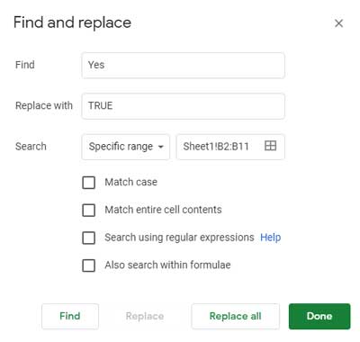
First, you must replace the value “Yes” with TRUE and “No” with FALSE. To do this, select the range B2:B, then go to Edit > Find and Replace.
In the “Find” field, type “Yes” (without quotes), and in the “Replace with” field, type TRUE. Choose “Specific range” in the “Search” field, then click “Replace all.”

Similarly, replace “No” with FALSE.
Next, select the range B2:B11 or up to the row where you want the tick boxes to appear. Go to the menu Insert > Tick box.
This is a quick way to replace “Yes” or “No” with TRUE or FALSE tick boxes in Google Sheets.
COUNTIFS with ‘<>’ and an Additional Condition from the Same Column
The COUNTIFS function with a ‘not blank’ condition and an additional criterion in the same column means applying two or more criteria to the same column.
This is often needed when you want to count all values in a column except blanks or specific selected values.
The following formula counts all non-blank cells in column A (range A2:A) except those with “Approved” or “Passed”:
=COUNTIFS(A2:A, "<>", A2:A, "<>Approved", A2:A, "<>Passed")Resources
- How to Count If Not Blank in Google Sheets [Tips and Tricks]
- COUNTIFS with Multiple Criteria in the Same Range in Google Sheets
- Google Sheets: COUNTIFS with Not Equal to in Infinite Ranges
- COUNTIFS in a Time Range in Google Sheets [Date and Time Column]
- COUNTIF | COUNTIFS Excluding Hidden Rows in Google Sheets
- How To Use COUNTIF or COUNTIFS In Merged Cells In Google Sheets
- Varying Array Sizes in COUNTIFS in Google Sheets
- OR Logic in Multiple Columns with COUNTIFS in Google Sheets
- OR Logic in COUNTIFS Across Either Column in Google Sheets
- COUNTIFS with ISBETWEEN in Google Sheets
- Counting XLOOKUP Results with COUNTIFS in Excel and Google Sheets


