If you want to look up values across a row and return a result from the same row or another row in the range, you can use the HLOOKUP function in Google Sheets. Of course, you could also use the LOOKUP function if the data is sorted by the first row in ascending order or the XLOOKUP function. If you’re more comfortable using HLOOKUP over the other two, you may find the advanced tip below helpful. Below, you’ll find examples of how to use multiple conditions in the HLOOKUP function in Google Sheets.

Sample Data

The sample data below shows the availability of different car types in a dealer’s various showrooms.

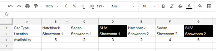
Car types such as Hatchback, Sedan, and SUV are in row 1, available locations are in row 2, and available quantities are in row 3.

You can use the following formula to look up “SUV” in row 1 and return the location available in row 2:

=HLOOKUP("SUV", A1:G3, 2, FALSE)

To return both the available location and quantity, you can use this formula:

=ARRAYFORMULA(HLOOKUP("SUV", A1:G3, {2, 3}, FALSE))

What if you want to find the availability of the “SUV” car type in “Showroom 2”? In this case, you need two conditions: one for “SUV” and one for “Showroom 2.”

The HLOOKUP function doesn’t directly support multiple conditions. Therefore, we need a workaround approach.

Example of Using Multiple Conditions in HLOOKUP

In the previous example, you can use the following formula to apply multiple conditions:

=ARRAYFORMULA(HLOOKUP(1, {(A1:G1="SUV")*(A2:G2="Showroom 2"); A3:G3}, 2, FALSE))

This formula is essentially searching for “SUV” in row A1:G1 and “Showroom 2” in A2:G2 and returning the value from the third row in the range.

However, you might see the search key as “1”, the range as {(A1:G1="SUV")*(A2:G2="Showroom 2"); A3:G3}, and the column index as “2”. This may seem confusing unless you understand the formula breakdown, which I will explain below.

How the Multiple Conditions HLOOKUP Works in Google Sheets (Formula Breakdown)

The formula follows this syntax:

HLOOKUP(search_key, range, index, [is_sorted])

Let’s break down the formula:

• Range: The range is {(A1:G1="SUV")*(A2:G2="Showroom 2"); A3:G3}.
  • (A1:G1="SUV"): This evaluates the first row for the value “SUV” and returns TRUE or FALSE.
  • (A2:G2="Showroom 2"): This evaluates the second row for the value “Showroom 2” and returns TRUE or FALSE.

When you multiply these two logical arrays, the result will be “1” wherever both conditions match, and “0” otherwise.

We combine this with the rest of the range (the vehicle availability data) using curly braces. The second row in the new range, A3:G3, contains the actual availability values, while the first row holds the logical results (1 or 0). Thus, the new range consists of only two rows.

• Search Key: We specify “1” as the search key because we’re looking for where both conditions are true (i.e., the cells in both rows match the search terms).
• Column Index: We specify 2 as the column index to return the value from the second row (which, in this case, is the available quantity).
• Is Sorted: We specify FALSE as the last argument since the data is not sorted.

Conclusion

We have now covered how to use multiple conditions in the HLOOKUP function in Google Sheets. By using this method, you can perform more complex lookups with multiple criteria across rows.

Note: The ARRAYFORMULA function is required here because the logical test in the range needs to be evaluated across multiple values.

Resources

• How to Return an Entire Column in HLOOKUP in Google Sheets
• How to Perform a Reverse HLOOKUP in Google Sheets
• LOOKUP, VLOOKUP, and HLOOKUP: Key Differences in Google Sheets
• VLOOKUP and HLOOKUP Combination In Google Sheets
• Transform Match Function to VLOOKUP or HLOOKUP in Google Sheets
• HLOOKUP to Search Entire Table and Find the Header in Google Sheets
• Move Single Column to Multiple Columns Using HLOOKUP in Google Sheets