For the functionality of the MINIFS array formula, we will pair it with the MAP Lambda function in Google Sheets. This is necessary because MINIFS typically returns only one minimum value per criteria set.

We’ll show practical examples using a diverse dataset with various value types. This helps you understand how to effectively use MINIFS with multiple criteria columns for expanded results.

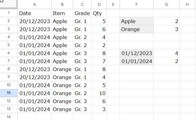
Refer to the screenshot below for the sample data, where column A contains sales dates (Date), column B contains fruit names (Item), column C contains fruit grades (Grade), and column D contains sales quantities (Qty).

Let’s delve into a few Google Sheets MINIFS arry formula formula examples.

MINIFS Array Formula: Basic Examples for Expanded Results

Example 1: Find the Lowest Sales Quantity of Apple and Orange

Steps:

• Specify the criteria, i.e., “Apple” and “Orange,” in cells F2 and F3, respectively.
• Insert the following MINIFS array formula in cell G2, which will return the results in G2:G3:

=MAP(F2:F3, LAMBDA(r, MINIFS(D1:D, B1:B, r)))

Note: Please scroll up to view the screenshot illustrating the input cells for criteria and the formula result in the cell range F2:G3.

Formula Explanation:

In the MINIFS formula, i.e., MINIFS(D1:D, B1:B, r), ‘r’ represents the current element, which will be F2 and F3 in corresponding rows.

The MAP function iterates over the criteria range F2:F3, allowing MINIFS to expand the results.

Example 2: Find the Lowest Sales Quantity in December 2023 and January 2024

Note: The source data includes a date column, not a month column. We will convert all the dates in the date column to the beginning of the month dates and use the starting dates (01/12/2023 and 01/01/2024) as criteria in the MINIFS array formula. This process is equivalent to finding the lowest values in those months.

Steps:

• Enter the criteria, 01/12/2023 and 01/01/2024, in cells F6 and F7, respectively.
• Enter the following MINIFS array formula in cell G6, which will return the results in G6:G7:

=ArrayFormula(MAP(F6:F7, LAMBDA(r, MINIFS(D1:D, EOMONTH(A1:A, -1)+1, r))))

Note: Please scroll up to view the screenshot illustrating the input cells for criteria and the formula result in the cell range F6:G7.

In the MINIFS function, EOMONTH(A1:A, -1)+1 converts the dates in column A to the beginning of the month date. The EOMONTH function requires the ARRAYFORMULA function to expand, and the MAP function iterates over the criteria range, similar to the previous example.

These are two basic examples of using the MINIFS function in an array formula in Google Sheets. Now, let’s explore some slightly more complex scenarios.

Advanced Examples

In the first example below, the MINIFS formula operates on criteria from two columns: fruit names and their corresponding grades.

It leverages an AND logic to return the lowest value that satisfies both the specified fruit name and its associated grade.

The second example also involves criteria from two columns, but it introduces OR logic within the grade column.

Here, the MINIFS formula returns the lowest value that matches the specified fruit name in one column and either of the grades listed in the other column.

Please see the two examples below.

AND Logic in MINFS Array Formula in Google Sheets

How can we determine the lowest sales quantity of Grade 1 Apple and Orange?

Steps:

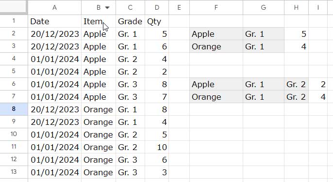
• Specify the “Apple” and “Orange” criteria in cell range F2:F3.
• Specify the criteria, “Gr. 1,” in cell range G2:G3.
• Insert the following MINIFS array formula in cell H2:

=MAP(F2:F3, G2:G3, LAMBDA(r_1, r_2, MINIFS(D1:D, B1:B, r_1, C1:C, r_2)))

Note: Please scroll up to view the screenshot illustrating the input cells for criteria and the formula result in the cell range F2:H3.

Formula Explanation:

In the MINIFS formula, i.e., MINIFS(D1:D, B1:B, r_1, C1:C, r_2), ‘r_1’ and ‘r_2’ represent the current pair of elements, which will be F2:G2 and F3:G3 in corresponding rows.

The MAP function iterates over the criteria range F2:G3, enabling MINIFS to expand the results.

OR Logic in MINFS Array Formula in Google Sheets

How can we determine the lowest sales quantity of Apple and Orange, considering they can be either Grade 1 or Grade 2?

The MINIFS function lacks built-in support for OR logic. To address this, we’ll employ a helper function to match grades and generate a column with TRUE for matches and FALSE for mismatches.

This approach satisfies MINIFS by using this formula as a virtual criteria column, with TRUE as the criterion. Consequently, there will only be one criterion from one column—a TRUE boolean value.

Steps:

1. Specify the “Apple” and “Orange” criteria in cell range F6:F7.
2. Specify the criteria, “Gr. 1,” in cell range G6:G7.
3. Specify the criteria, “Gr. 2,” in cell range H6:H7.
4. Insert the following MINIFS array formula in cell I6:

=ArrayFormula(MAP(F6:F7, G6:G7, H6:H7, LAMBDA(r_1, r_2, r_3, MINIFS(D1:D, B1:B, r_1, REGEXMATCH(C1:C, r_2&"|"&r_3), TRUE))))

Note: Please scroll up to view the screenshot illustrating the input cells for criteria and the formula result in the cell range F6:I7.

Formula Explanation:

In the MINIFS formula, i.e., MINIFS(D1:D, B1:B, r_1, REGEXMATCH(C1:C, r_2&"|"&r_3), TRUE), ‘r_1’ and TRUE represent the current pair of elements, which will be {F6, TRUE}, and {F7, TRUE} in corresponding rows.

The REGEXMATCH function matches the grades (i.e., r_2&"|"&r_3) in the corresponding column C1:C, returning either TRUE or FALSE. Here, ‘r_2’ and ‘r_3’ represent the current pair of elements, which will be G6 and H6 in the first row and G7 and H7 in the second row.

The pipe “|” is used to separate each criterion. For adding more criteria as part of the OR logic, you can use it as r_2&"|"&r_3&"|"&next_criterion.

This setup allows for a partial and case-sensitive match of grades. To make it case-insensitive, use "(?i)"&r_2&"|"&r_3 pattern, and for an exact match, use "(?i)^"&r_2&"$|^"&r_3&"$" pattern.

Conclusion

Above, you can see four MINIFS array formula examples using the MAP lambda function. They are unique in terms of functionality as I have included multiple conditions using both AND and OR logic.

How do we find the highest values instead of the lowest values conditionally? Here are the relevant tutorials:

1. MAXIFS Function in Google Sheets: Find Maximum Value Conditionally.
2. Master MAXIFS Array Formulas in Google Sheets: The Ultimate Guide.