This post is not about the Matches Regular Expression match in Query. It’s about how to use the Match function in Query Where clause in Google Sheets.

No doubt, the Match is one of the useful functions in all the popular Spreadsheet applications. It’s for returning the position of a string, date, or number value in a single row range or single column range.

The position (called relative position) returned by the Match formula can be used as an expression in other functions. Here that ‘other functions’ is the Query.

Yes! Here we will make use of the Match feature, i.e. get the position of an item in a single row, in Query. The purpose?

When we use the Match function in the Query Where clause in Google Sheets, the purpose is to search the column to filter instead of directly specifying the column.

Please go through the data below.

It’s a sample “Attendance” sheet in which the first row contains a few names (employees or students) and below their present/absent/holiday (attendance) status.

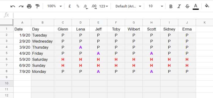
I want to filter the data for “Scott”, not all the data but the days he was absent (represented by “A”).

Here I am going to use the Match function within Query Where clause to solve the problem.

We can use a single Match or multiple Math functions in the Query Where clause in Google Sheets depending on the number of columns to filter.

In the above case, we only want to use a single Match function.

Single Match Function in Query Where Clause in Google Sheets

Before including the Match function in the Query where clause, let’s see how we will normally use the formula in this case.

Using the below Query formula we can filter the data for the absent days for “Scott”.

=query(
     A1:J,
     "Select * where H='A'",1
)

Here there is no scope of including the Match function in the Where clause. Let’s see an alternative to the above formula.

First, count the columns from the left to right in the data until reaches “Scott” in row # 1. You will get the number 8 (column H), right?

By using the data as an expression (by surrounding the data by Curly Braces), we can use column numbers in the Where clause.

=query(
     {A1:J},
     "Select * where Col8='A'",1
)

This makes us to possible to use the below Match function. How?

=match("Scott",A1:J1,0)

The above formula will return the column number 8 corresponding to the name “Scott”. We can replace 8 in the above Query formula with the just above Match formula.

=query(
     {A1:J},
     "Select * where Col"&match("Scott",A1:J1,0)&"='A'",1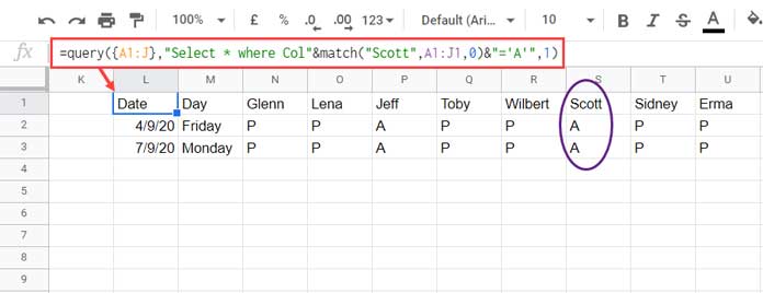
)

Note: If you just want the date column, replace "Select * with "Select Col1.

If the Match criterion, i.e. “Scott”, is a cell reference, assume in cell K1, then use the formula as below.

=query(
     {A1:J},
     "Select * where Col"&match(K1,A1:J1,0)&"='A'",1
)

Multiple Match Functions in Query Where Clause in Google Sheets

Suppose you want to test whether two of your employees were absent on the same day. Then you may want to use multiple Match functions in the Query Where clause in Google Sheets.

Here I am considering the employees “Jeff” and “Scott”.

=query(
     {A1:J},
     "Select * where Col"&match("Scott",A1:J1,0)&"='A' and Col"&match("Jeff",A1:J1,0)&"='A'",1
)

I have used two match formulas in the Where clause as well as the AND Query logical operator.

Alternative Formulas (Filter and Query Itself)

If you just want to filter the records for one employee, here “Scott”, you can of course consider using alternative formulas. No doubt, Filter tops the chart.

=filter(
     A1:J8,
     filter(
        A1:J8,A1:J1="Scott"
     )="A"
)

The inner Filter formula filters the 8th column based on the name “Scott”.

The outer Filter formula filters the table if the 8th column contains the letter “A”.

You can find more details here – Two-way Filter in Google Sheets [Dynamic Vertical and Horizontal Filter].

To improve your Google Sheets skill, I’m providing you one more formula. It’s actually using Query with Transpose.

=Query(
     {transpose(query(transpose(A1:J),"Select * where Col1='Scott'")),A1:J},
     "Select Col2 where Col1='A'"
)

Explanation (Query Transpose)

The Transpose, i.e. transpose(A1:J), changes the orientation of the data so the employee names will be in the first column in the transposed data.

The Query selects the row that contains the name “Scott” in the first column.

query(transpose(A1:J),"Select * where Col1='Scott'")

I have once again transposed this data. So we have the 8th column with us.

transpose(query(transpose(A1:J),"Select * where Col1='Scott'"))

Added the entire data as the adjoining columns to the right side of the 8th column.

{transpose(query(transpose(A1:J),"Select * where Col1='Scott'")),A1:J}

The outer Query filters the first column if it contains “A”.

Because of this (the first column contains names then all the eight columns), I have started the Select clause in the outer Query like "Select Col2 instead of "Select Col1.

It will return the date column only.

For all the columns, you may need to specify the Where clause in the outer Query like "Select Col2, Col3, Col4...

That’s all about how to use the Match function in Query Where clause in Google Sheets.

Thanks for the stay. Enjoy!

Resources:

1. Dynamic Column Id in Query Importrange Using Named Ranges.
2. How to Get Dynamic Column Reference in Google Sheets Query.
3. Dynamic Formula to Select Every nth Column in Query in Google Sheets.