Lookup by Keyword in a Phrase in Google Sheets

Sometimes, your data contains full sentences or descriptive phrases, while your lookup table consists of individual keywords. For example, you might have a phrase like “Black Friday Shoes Sale”, and you want to match it against a list of keywords like “Shoes”, “Jackets”, or “Discounts” — then return the associated category such as Footwear, Apparel, or Promotions.

While standard lookup functions like VLOOKUP or XLOOKUP can support partial matches using wildcards, they expect the search key to be the keyword and the table to contain longer values. In our case, it’s the other way around — the phrase is the input, and the keyword is buried within it.

In this tutorial, you’ll learn how to look up a keyword found inside a longer phrase in Google Sheets using three flexible and powerful formula techniques. These approaches use functions like LET, REGEXMATCH, REGEXEXTRACT, and COUNTIF to make your lookups smarter. Whether you’re building a tagging system, categorizing marketing campaigns, or detecting named entities, these solutions have you covered.

Table of Contents

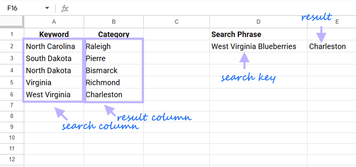
Sample Data: Keywords and Categories

Here’s the lookup table we’ll use:

Keyword	Category
North Carolina	Raleigh
South Dakota	Pierre
North Dakota	Bismarck
Virginia	Richmond
West Virginia	Charleston

And here’s an example phrase:

Search Phrase: West Virginia Blueberries

Your goal is to detect which keyword (like “West Virginia”) appears inside the phrase and return its associated category — in this case, “Charleston”.

Keyword lookup phrase example with search key in D2 and keyword-category table in A2:B

Why Standard VLOOKUP Doesn’t Work for Keyword Lookups

Let’s try a few basic formulas to understand the limitation.

=VLOOKUP("West Virginia Blueberries", A2:B, 2, FALSE)

This will return #N/A — because there’s no exact match in column A.

Now try this:

=VLOOKUP("West Virginia", A2:B, 2, FALSE)

This works only if you already know the correct keyword.

Even wildcards won’t help:

=VLOOKUP("*West Virginia Blueberries*", A2:B, 2, FALSE)

This doesn’t work because VLOOKUP only supports wildcards when the lookup range contains full values that match the wildcard pattern in the search key. In our case, the keyword “West Virginia” is just a part of the phrase — and the phrase doesn’t exist in column A.

So to make this work, we need to reverse the logic: instead of trying to match the phrase to the table, we scan the table to see which keyword it contains.

This is where lookup by keyword in a phrase in Google Sheets becomes essential.

Method 1: REGEXMATCH and FILTER

=LET(
   reg, ARRAYFORMULA((LEN($A$2:$A) > 0) * REGEXMATCH(LOWER(D2), LOWER($A$2:$A))),
   x, FILTER($B$2:$B, reg),
   y, FILTER(LEN($A$2:$A), reg),
   CHOOSEROWS(SORT(x, y, 0), 1)
)

Formula Explanation:

reg, ARRAYFORMULA((LEN($A$2:$A) > 0) * REGEXMATCH(LOWER(D2), LOWER($A$2:$A)))
→ This checks if each non-empty keyword in A2:A exists inside D2. It returns 1 only where there’s a match and the keyword cell isn’t blank. LOWER ensures case-insensitive comparison.
x, FILTER($B$2:$B, reg)
→ Picks the categories from column B where the match is TRUE — here that’s “Richmond” and “Charleston”.
y, FILTER(LEN($A$2:$A), reg)
→ Filters the lengths of the matched keywords — “Virginia” (8), “West Virginia” (13)
CHOOSEROWS(SORT(x, y, 0), 1)
→ Sorts the matched categories by keyword length in descending order, and picks the first one. So we get the category for the longest match — in this case, “Charleston” for “West Virginia”.

How to Apply to a Column of Phrases

=MAP(D2:D, LAMBDA(r,
 LET(
   reg, ARRAYFORMULA((LEN($A$2:$A) > 0) * REGEXMATCH(LOWER(r), LOWER($A$2:$A))),
   x, FILTER($B$2:$B, reg),
   y, FILTER(LEN($A$2:$A), reg),
   CHOOSEROWS(SORT(x, y, 0), 1)
 ))
)

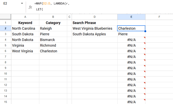
Method 1 result: REGEXMATCH and FILTER returning category for longest keyword match

To remove #N/A errors, wrap the formula with IFNA(...).

Method 2: REGEXEXTRACT and VLOOKUP

=LET(
   reg, ARRAYFORMULA(IFNA(REGEXEXTRACT(LOWER(D2), LOWER($A$2:$A)))),
   key, FILTER(reg, LEN(reg)=MAX(LEN(reg))),
   VLOOKUP(key, $A$2:$B, 2, FALSE)
)

Formula Explanation:

reg, ARRAYFORMULA(IFNA(REGEXEXTRACT(LOWER(D2), LOWER($A$2:$A))))
→ This returns the keywords that are found in the phrase — not just TRUE/FALSE. Any non-matches become blank because of IFNA.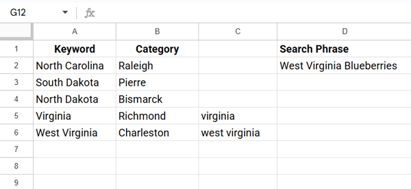
key, FILTER(reg, LEN(reg)=MAX(LEN(reg)))
→ This keeps only the longest matched keyword. So if both “Virginia” and “West Virginia” are matched, this picks “West Virginia”.
VLOOKUP(key, $A$2:$B, 2, FALSE)
→ Standard VLOOKUP using the matched keyword to return the category — here, “Charleston”.

How to Apply to a Column of Phrases

=MAP(D2:D, LAMBDA(r,
 LET(
   reg, ARRAYFORMULA(IFNA(REGEXEXTRACT(LOWER(r), LOWER($A$2:$A)))),
   key, FILTER(reg, LEN(reg)=MAX(LEN(reg))),
   VLOOKUP(key, $A$2:$B, 2, FALSE)
 ))
)

To remove #N/A errors, wrap the formula with IFNA(...).

Method 3: COUNTIF and Wildcards

=LET(
   count, ARRAYFORMULA((LEN($A$2:$A) > 0)*(COUNTIF(D2, "*"&$A$2:$A&"*"))),
   x, FILTER($B$2:$B, count),
   y, FILTER(LEN($A$2:$A), count),
   CHOOSEROWS(SORT(x, y, 0), 1)
)

Formula Explanation:

count, ARRAYFORMULA((LEN($A$2:$A) > 0) * (COUNTIF(D2, "*"&$A$2:$A&"*"))) → This checks if each non-empty keyword in A2:A appears somewhere inside D2. It returns 1 where matched, and 0 otherwise. Matching ones return 1.
x, FILTER($B$2:$B, count)
→ Gets the categories where the keyword matched — just like in Method 1..
y, FILTER(LEN($A$2:$A), count)
→ Pulls the lengths of the matched keywords.
CHOOSEROWS(SORT(x, y, 0), 1)
→ Sorts by length and returns the category corresponding to the longest match.

How to Apply to a Column of Phrases

=MAP(D2:D, LAMBDA(r,
 LET(
   count, ARRAYFORMULA((LEN($A$2:$A) > 0)*(COUNTIF(r, "*"&$A$2:$A&"*"))),
   x, FILTER($B$2:$B, count),
   y, FILTER(LEN($A$2:$A), count),
   CHOOSEROWS(SORT(x, y, 0), 1)
 ))
)

To remove #N/A errors, wrap the formula with IFNA(...).

Which Formula Should You Use?

Formula Approach	Supports Longest Match	Uses Regex	Simple to Maintain
REGEXMATCH	✅	✅	✅
REGEXEXTRACT	✅ (most accurate)	✅	❌
COUNTIF	✅	❌	✅

If you want a regex-free and simple solution, use COUNTIF. For those comfortable with regex, REGEXMATCH and REGEXEXTRACT offer similar precision — all three methods correctly handle overlapping keywords by prioritizing the longest match.

Copy Sample Sheet