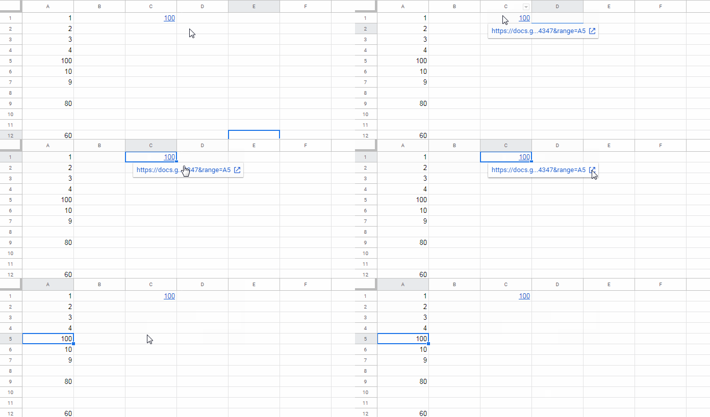
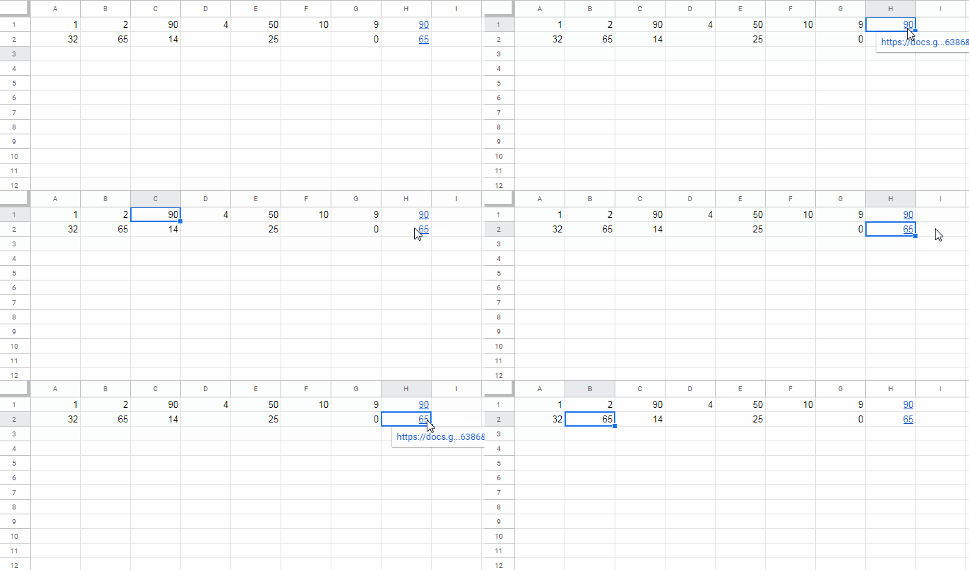
Hyperlink to Max or Min Value in Google Sheets

You can create a dynamic hyperlink to the max or min value in a row or column in Google Sheets using a combination of functions: XLOOKUP, REGEXREPLACE, HYPERLINK, and either MAX or MIN.

This tutorial shows you how to find and hyperlink to the maximum or minimum value in a selected range.

Steps to Create a Hyperlink to Max or Min Value

Open the Sheet that contains the data where you want to find the max or min value.
Right-click any cell (e.g., cell A1) to open the context menu.
Select View more cell actions > Get link to this cell.
Paste the link into any empty cell. It will look like this:
https://docs.google.com/spreadsheets/d/1ByjWyXJ3h5bLCTiN9p7Iev8exasjtQRl5GPLzl2U-J4/edit?gid=1800049113#gid=1800049113&range=A1
Remove the cell reference (e.g., A1) from the end of the URL, so you’re left with just:
https://docs.google.com/spreadsheets/d/1ByjWyXJ3h5bLCTiN9p7Iev8exasjtQRl5GPLzl2U-J4/edit?gid=1800049113#gid=1800049113&range=

Get the Relative Cell Reference of the Max or Min Value

Use this formula to return the relative address (e.g., A12) of the max value in a column:

=REGEXREPLACE(CELL("address", XLOOKUP(MAX(A1:A), A1:A, A1:A)), ".*!|\$", "")

Replace A1:A with your target column or row.
To find the minimum value instead, simply replace MAX with MIN.

Combine the URL and the Cell Address

Now, append the relative address to the trimmed URL:

"https://docs.google.com/spreadsheets/d/1ByjWyXJ3h5bLCTiN9p7Iev8exasjtQRl5GPLzl2U-J4/edit?gid=1800049113#gid=1800049113&range=" & REGEXREPLACE(CELL("address", XLOOKUP(MAX(A1:A), A1:A, A1:A)), ".*!|\$", "")

Create a Clickable Link

Wrap the above in a HYPERLINK formula to make it clickable:

=HYPERLINK("https://docs.google.com/spreadsheets/d/1ByjWyXJ3h5bLCTiN9p7Iev8exasjtQRl5GPLzl2U-J4/edit?gid=1800049113#gid=1800049113&range=" & REGEXREPLACE(CELL("address", XLOOKUP(MAX(A1:A), A1:A, A1:A)), ".*!|\$", ""), "Jump to Max")

To hyperlink to the min value, replace MAX with MIN and adjust the link label if needed.

Use Cases:

Hyperlink to Max or Min Value in a Column in Google Sheets

Modify the formula to match your target column range. Use MAX to link to the highest value and MIN to jump to the lowest value in that column.

Example of Hyperlinking Max or Min Values in a Column in Google Sheets

Hyperlink to Max or Min Value in a Row in Google Sheets

Change the formula range to a row (e.g., A1:Z1). Use MAX for the largest value and MIN for the smallest value in the row.

Example of Hyperlinking Max or Min Values in a Row in Google Sheets

Formula Breakdown

Here’s how the formula works:

=REGEXREPLACE(CELL("address", XLOOKUP(MAX(A1:A), A1:A, A1:A)), ".*!|\$", "")

MAX(A1:A): Finds the maximum value in the range.
XLOOKUP(MAX(A1:A), A1:A, A1:A): Returns the cell containing the max value.
CELL("address", ...): Gets the absolute reference of that cell (like $A$12).
REGEXREPLACE(..., ".*!|\$", ""): Strips the sheet name and dollar signs to return a relative reference like A12.

Replace MAX with MIN for linking to the minimum value.

Conclusion

With this method, you can easily create a hyperlink to the max or hyperlink to the min value in any row or column of your Google Sheets. It’s especially helpful in large datasets where you want to jump to key values with a single click.