


We can use the Product function in Google Sheets to return the product of a series of numbers. Product is that what returns when two or more values are multiplied together.
We can use the * (asterisk) operator for returning the product of values, but it’s not a perfect alternative to this function.
If you use only two values (factor 1 and factor 2), then you can use the Product, Asterisk operator, or the Multiply function.
If there are more values, then using the Product function is suggestible. I’ll come to this point later.
In this post you can learn how to use the Product function in Google Sheets. Also find some other tips like using Filter function with Product to filter out 0’s or ‘limit to a range’.
PRODUCT Function – Syntax and Arguments
Syntax:
PRODUCT(factor1, [factor2, …])Arguments:
- factor1 – The first number or array to calculate for the product.
- factor2, … – Additional values to multiply by.
The facor1, factor2, factor3…factor30 are the numbers to multiply together.
The specified number of arguments that the PRODUCT function can take is 30. But, as per the official documentation, it would take an arbitrary number of arguments.
Here are a few examples that can simplify the use of this ‘Maths’ category function.
Example
=product(5,10,2)The above formula would return 100 which is equal to using the below formula.
=5*10*2When you use the numbers 5, 10, and 2 within the formula as above there is no difference in using the Product function with the asterisk operator. Both are equally time taking to code.
But if the arguments (numbers) are cell references, using the Product function is far better than using the asterisk operator.
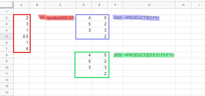
The below examples (please see the below image for formulas) will clear this point.
Note:
The Product formula in Google Sheets will ignore text strings, TRUE/FALSE Boolean values, and blank cells in the array. But it will consider both the date and time.
Further the array can be of different size. Please see example three (in green color).
Why Multiply Function or Asterisk Operator is Not an Equivalent?
If you have followed the examples on the screenshot, you can understand why we can’t replace the Product function with the asterisk operator.
For example, if we replace the B2 formula, it would be like this using the asterisk operator.
=A2*A3*A4*A5*A6*A7So if the number of arguments is large, it’s is not practical to follow this method.
Regarding the function Multiply, its for returning the product of only two numbers or for multiplying one array with another array. See the below two multiplication formulas.
Multiplication Formulas
Example 1:
=MULTIPLY(5,10)Result: 50
Example 2:
| A | B | C | |
| 1 | Quantity | Rate | Amount |
| 2 | 5 | 10 | 50 |
| 3 | 4 | 20 | 80 |
| 4 | 6 | 30 | 180 |
Here in C2, we can use either of the below to formulas not Product.
Formula 1:
=ArrayFormula(multiply(A2:A4,B2:B4))Formula 2:
=ArrayFormula(A2:A4*B2:B4)Product Function with Filter Function in Google Sheets (Conditional Product)
Other than numbers and cell references, the arguments in Google Sheets Product function can be an expression. That means we can use a formula as an argument.
Assume I want to find the product of numbers between 1 and 3 (both inclusive) provided in the range A1:A. So I’ll use the Filter function to filter out other values and then find the product.
=product(filter(A1:A,A1:A>=1,A1:A<=3))If any of the arguments in the product are 0, then the output will be 0. Using the Filter, we can filter out 0 values in the Product calculation.
=product(filter(A1:A,A1:A>0))That’s all. Enjoy!
Related Reading: