The IF function in Google Sheets allows you to compare a value with what you expect, called a logical expression. This expression can result in either TRUE or FALSE.
An example of a logical expression is =A1="Apple", which will return TRUE if A1 contains “Apple” and FALSE otherwise.
What makes the IF function more useful is its ability to return outputs based on the outcome of the logical expression. You can specify what value you want the function to return or what calculation it should perform if the expression is TRUE, and what it should return or do if it’s FALSE.
For more complex scenarios, you can use nested IF statements. This involves placing additional IF statements within the value_if_false argument of the previous IF statement. Nested IFs allow you to create formulas with multiple conditions.
Syntax: IF(logical_expression, value_if_true, value_if_false)
In this tutorial, we’ll check out the basics of the IF function and dive into using nested IF statements to really get the most out of conditional logic in Google Sheets.
Basic Examples
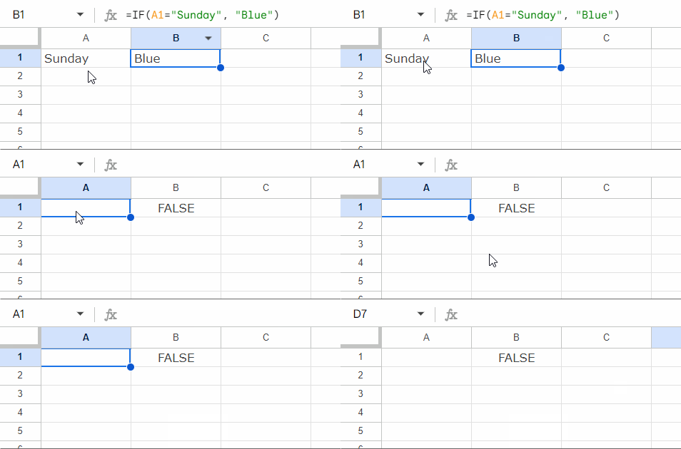
Enter the text “Sunday” in cell A1 and the following formula in cell B1:
=IF(A1="Sunday", "Blue")It will return “Blue”. If you delete the value in cell A1 or enter any other text, the formula will return the default value, which is FALSE. This means the value_if_false argument is optional in the IF function in Google Sheets.

Let’s see a different formula:
=IF(A1="Sunday", "Blue", "Grey")This will return “Blue” if A1 is “Sunday”, otherwise it will return “Grey”.
Logical expressions can include comparison operators such as greater than (>), less than (<), not equal to (<>), greater than or equal to (>=), less than or equal to (<=), and equals (=) when working with numeric, date, or time values.
For example, the date in cell A1 is June 15, 2030. So the following formula will return “Operational”:
=IF(A1 <= DATE(2025, 12, 31), "Expired", "Operational")The date function in the logical expression follows the syntax DATE(year, month, day).
In the following example, with the same date in cell A1, the formula will return ‘Operational’ until the current calendar date (as per the system) passes June 15, 2030:
=IF(A1 < TODAY(), "Expired", "Operational")This formula checks if the date in cell A1 is before today’s date (TODAY()). If it is, it returns ‘Expired’; otherwise, it returns ‘Operational’.”
Nested IF Functions in Google Sheets
As mentioned earlier, nested IFs allow you to create formulas with multiple conditions. You can place additional IF statements within the value_if_false argument of the previous IF statement.
This is a very useful technique, and mastering it is essential, although there is a better alternative function for this called IFS.
You can understand how to use nested IF functions with the following syntax:
IF(logical_expression, value_if_true, IF(logical_expression, value_if_true, IF(logical_expression, value_if_true, value_if_false)))Ensure the formula has closing brackets that match the number of nested IF functions or logical expressions.
Example:
Consider the following formula:
=IF(A1>80, "Diamond", IF(A1>50, "Platinum", IF(A1>30, "Silver", "Unknown")))In this formula, there are three logical expressions and three closing brackets.
The formula returns:
- “Diamond” if the value in cell A1 is greater than 80,
- “Platinum” if the value in cell A1 is greater than 50 but not greater than 80,
- “Silver” if the value in cell A1 is greater than 30 but not greater than 50,
- “Unknown” if the value in cell A1 is 30 or less.
Examples of IF and ARRAYFORMULA Combination in Google Sheets
When you specify an array reference in the logical expression part of the IF function, you should use the ARRAYFORMULA function or other array functions alongside it in Google Sheets.
For example, the following formula will return the month number from the dates in A2:A:
=ArrayFormula(IF(A2:A<>"", MONTH(A2:A), ""))It returns an empty string (“”) in empty rows.

If you see an array reference in logical expressions and no ARRAYFORMULA in use, that means it might be used within array functions such as INDEX, SORT, SORTN, or FILTER.
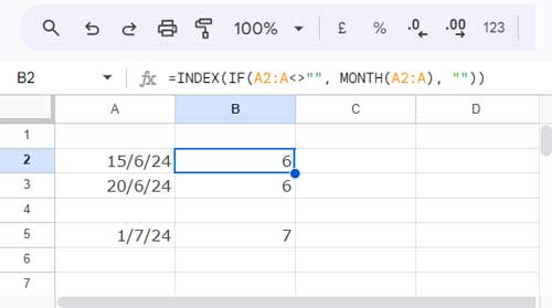
For example, you can replace the ARRAYFORMULA in the above formula with INDEX as follows:
=INDEX(IF(A2:A<>"", MONTH(A2:A), ""))


1. How can I copy-paste a formula with just the same one cell by not changing the formula if pasted?
2. How to create an aging deducting the completion?
Hi, Venus,
1. Use absolute reference in your formula. For example use
=sum($A$1:$A$5)instead of=sum(A1:A5).2. Please share a sample Sheet URL below.
When A1 is populated B1 should be auto-populated with today’s date. When I open the google spreadsheet tomorrow, B1 should still have today’s date.
Is there a formula for this? I’m using a tablet to create Google Spreadsheet. Thanks!
Hi, Carlton Robinson,
That’s not possible with a built-in function in Google Sheets. Probably that can do with a custom function called OnEdit. Find that script by following the link below.
https://developers.google.com/apps-script/guides/triggers/
If that is not helping, please post your question on the Google Docs official community forum HERE. Because I am not familiar with Script 🙁
Best,
Hi!
Congrats for this amazing site!
I’m really a noob and would really appreciate you to help me with the issue below.
1. There’s a column with different texts.
2. I need to categorize every text with different specific tags in another column.
3. For instance: if A2 contains “WordA” then write “A” in B2; if A2 contains “WordB” then write “B” in B2, and so on (up to 10 different tags).
Is this possible?
Thanks in advance!
Welcome!
I am glad to hear that you liked this site.
Regarding the problem, you can use IF, IFS or CHOOSE. I prefer the function CHOOSE here. Try this formula in cell B2.
=switch(A2,"WordA","A","WordB","B","WordC","C")You can easily add more conditions to it.
For an entire column range A2:A, just apply the below formula in B2.
=iferror(switch(A2:A,"WordA","A","WordB","B","WordC","C"))Thanks!
Dear Sir,
How can write Google Sheet Function for Average Volume-10 days of NSE Stock
Hi Sangita,
Welcome to Info Inspired!
Here is a sample formula.
I think this formula can find the average volume of the provided ticker. You can change the ticker and date duration.
Note:
1. Please re-type the double quotes in formula.
2. Learn Googlefinance function.
Thanks.