In this post, let’s learn to highlight consecutive or adjacent duplicates in Google Sheets.

The conditional formatting for the same is simple.

Sometimes we may require to find duplicate values in rows or columns in consecutive cells, not in distant cells.

I’ve conditional format rules for the same for both row and column-wise data.

That will help you identify such values.

For example, we have the text “apple” in cells A2, A4, A5, and A7. The formula should only highlight A4 and A5 since those are the consecutive cells with duplicates.

You can also decide whether to conditional format both A4 and A5 or A5 alone, i.e., from the second occurrence onwards.

Here are examples of highlighting adjacent duplicates in Google Sheets.

Highlight Adjacent Duplicates Row or Column-Wise

In the first example, we will use a conditional format custom formula rule to highlight all the occurrences of duplicates in consecutive cells.

Later we can see how to exclude the first occurrence.

Highlight All the Occurrence of Consecutive Duplicate Cells

Please see the screenshot below.

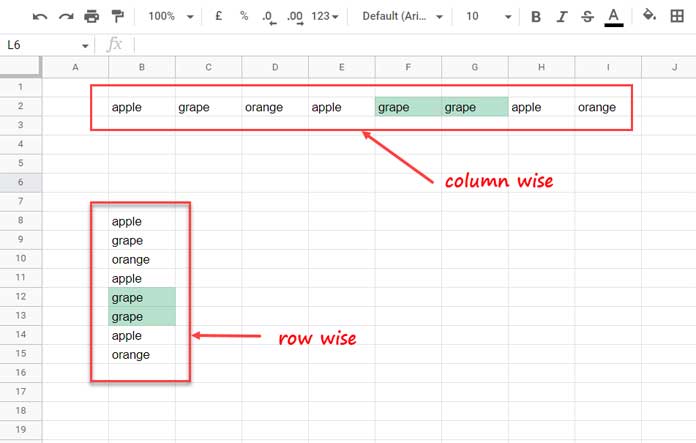
Column-Wise Data

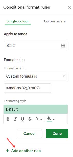
We can use the following LEN and Logical AND based rule for the column-wise data in B2:I2.

=and(len(B2),B2=C2)

You must apply this twice, first for the range B2:I2 and then for the range C2:I2. Here is how?

Go to Format > Conditional formatting.

It will open the sidebar panel to enter the range of cells to highlight. Also, to add the above formula rule.

Find “Apply to range,” and enter B2:I2, which is the range to highlight for consecutive or adjacent duplicated cells.

Then select “Custom formula is” under “Format rules.”

Just enter the above formula and choose the color to fill the cells that contain the adjacent duplicate values.

Below that, find the option “Add another rule.”

Open that and modify “Apply to range” to C2:I2 and “DONE.”

Note:- To include another row, i.e., B3:I3, you are only required to modify the “Apply to ranges” B2:I2 and C2:I2 to B2:I3 and C2:I3, respectively.

Row-Wise Data

We can follow the above method when we want to highlight adjacent duplicates in rows in Google Sheets.

Please see the range B8:B15 on screenshot # 1 above.

We can use the following conditional format formula for B8:B15 and B9:B15 (twice as above)

=and(len(B8),B8=B9)

Note:- When you have one more column, i.e., C8:C15, just modify the “Apply to range” to B8:C15 and B9:C15.

Highlight Adjacent Duplicates Except for First Occurrence

Please see screenshot # 3 below.

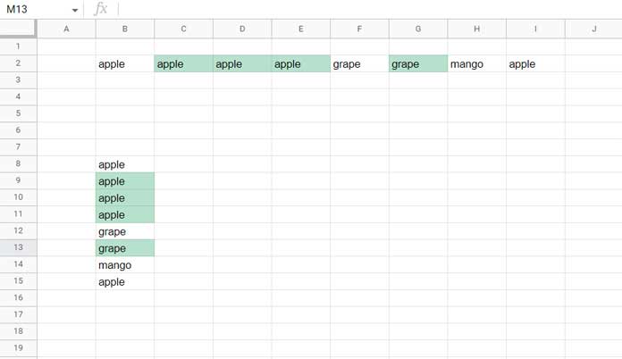
You can see the difference!

The consecutive duplicate cells are highlighted, both in column-wise and row-wise data, except for the first occurrence.

We require to delete one rule to achieve this.

Horizontal Data:- Delete the rule added for B2:I2. We only require the C2:I2 one.

Vertical Data:- Delete the rule added for B8:B15. We only require the B9:B15 one.

This way we can highlight adjacent duplicates in Google Sheets.

That’s all. Thanks for the stay. Enjoy!

Resources

• Date Related Conditional Formatting Rules in Google Sheets.
• Find All the Cells Having Conditional Formatting in Google Sheets.
• Highlight Duplicates in Single, Multiple Columns, All Cells in Google Sheets.
• How to Highlight Cells Based on Expiry Date in Google Sheets.
• Highlight Visible Duplicates in Google Sheets.
• Relative Reference in Conditional Formatting in Google Sheets.
• Compare and Highlight Up and Down in Ranking in Google Sheets.
• Highlight Top 10 Ranks in Single or Each Column in Google Sheets.
• How to Include Adjacent Blank Cells in Sumif Range in Google Sheets.
• Google Sheets – Vlookup Adjacent Cells.