Grouping a column in Google Sheets is easier than you might think. All you need is a basic understanding of the QUERY function. However, sometimes you may want to group data based on the first few characters in a column. Let me explain how to do that step by step.
When working with spreadsheet applications, the best way to generate ideas is by learning as many functions as possible. This is because you can combine or nest functions to achieve your desired results.
For grouping a column by the first few characters, you’ll need to use a combination of functions—specifically, the LEFT and QUERY functions.
Sample Data for Grouping by the First Few Characters
The sample data consists of item codes in the first column and spans across 4 columns.
| Item Code | Product | Unit | Qty |
| AE2565 | Apple – U.S. Fancy | Kg | 10 |
| AE2566 | Apple – U.S. No. 1 | Kg | 5 |
| AE2567 | Apple – U.S. Utility | Kg | 10 |
| AE2566 | Apple – U.S. No. 2 | Kg | 10 |
| OE1979 | Orange – U.S. Fancy | Kg | 20 |
| OE1980 | Orange – U.S. No. 1 | Kg | 20 |
| OE1982 | Orange – U.S. No. 1 Golden | Kg | 10 |
In this dataset, the goal is to group the data based on the first two letters in column A and sum the quantities in column D.
A standard QUERY formula that groups by item codes would look like this:
=QUERY(A1:D, "SELECT Col1, SUM(Col4) WHERE Col1<>'' GROUP BY Col1", 1)But how do you group this data by the first few characters of the item codes? Let’s learn how to do it step by step.
Step 1: Extracting the First Few Characters
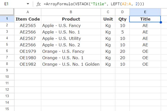
Our original data is in the range A1:D, where A1:D1 contains the field labels. In cell E1, enter the following array formula to extract the first two characters from the item codes:
=ArrayFormula(VSTACK("Title", LEFT(A2:A, 2)))
The LEFT function returns the first two characters from the range A2:A, and the VSTACK function appends the column name “Title” to it. You can replace “Title” with any name you prefer, such as “Group Item.”
Step 2: Grouping Data by the First Two Characters
Next, extend the data range to include column E and group by column E instead of column A. The formula will be:
=QUERY(A1:E, "SELECT Col5, SUM(Col4) WHERE Col5<>'' GROUP BY Col5", 1)This will group the data by the first two characters. If you enter this formula in cell G1, you will get the output in the range G1:H3.
| Title | sum Qty |
| AE | 35 |
| OE | 50 |
Step 3: Removing the Helper Column
If you prefer not to keep the helper column, modify the data used in the QUERY function.
Currently, the data range is A1:E. You should use it as follows:
HSTACK(ArrayFormula(VSTACK("Title", LEFT(A2:A, 2))), B1:D)The HSTACK function horizontally stacks the helper column formula with the data in B1:D.
You can use this formula with the standard QUERY formula mentioned above Step 1 as follows:
=QUERY(HSTACK(ArrayFormula(VSTACK("Title", LEFT(A2:A, 2))), B1:D), "SELECT Col1, SUM(Col4) WHERE Col1<>'' GROUP BY Col1", 1)Note: You can move the ARRAYFORMULA to the beginning, which is a common practice. The formula would then look like this:
=ArrayFormula(QUERY(HSTACK(VSTACK("Title", LEFT(A2:A, 2)), B1:D), "SELECT Col1, SUM(Col4) WHERE Col1<>'' GROUP BY Col1", 1))That’s how you group data by the first few characters in Google Sheets.
Resources
- How to Remove the First N Characters in Google Sheets
- How to Group Data by Month and Year in Google Sheets
- Group and Average Unique Column in Google Sheets
- How to Group Rows and Columns in Google Sheets
- Formula to Group Dates by Quarter in Google Sheets
- Group and Sum Time Duration Using Google Sheets Query
- Formula to Insert Group Total Rows in Google Sheets
- Group and Sum Data Separated by Blank Rows in Google Sheets


