To autofill days of the week, you can use either an array formula or a built-in feature in Google Sheets. When employing the formula, you can exclude specific weekends, making it even more advantageous.

In this tutorial, I’ll also show you how to easily insert blank rows below days of the week. Let’s begin by exploring the built-in feature.

Autofill Days of the Week Using the Built-in Feature

Assuming you want to autofill days of the week starting from cell A1 down the column, follow these steps:

1. Type the first day of the week you want to appear in a cell, such as entering “Monday” or “Mon” in cell A1.
2. Click and drag the blue square (fill handle) in the lower-right corner of cell A1 down as far as you want to fill the remaining cells with consecutive days.

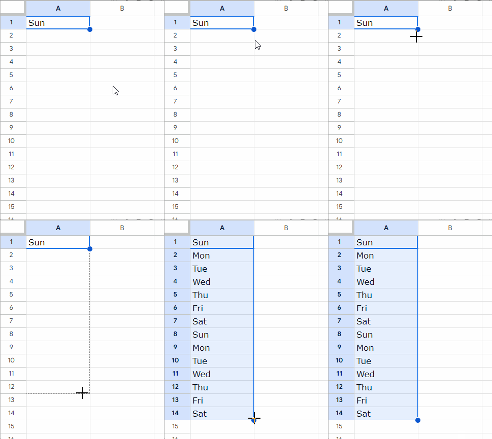
This is the easiest method to autofill the days of the week in a column in Google Sheets. To get it in a row, drag the fill handle across the row.

If you want blank rows between each day of the week, follow the example below:

1. Enter “Monday” or “Mon” in cell A1.
2. Select A1 plus as many blank cells as you want below that. For instance, if you want two blank rows below each day of the week, select A1:A3.
3. Drag the fill handle (blue square) in the lower-right corner of cell A3 as far as you want.

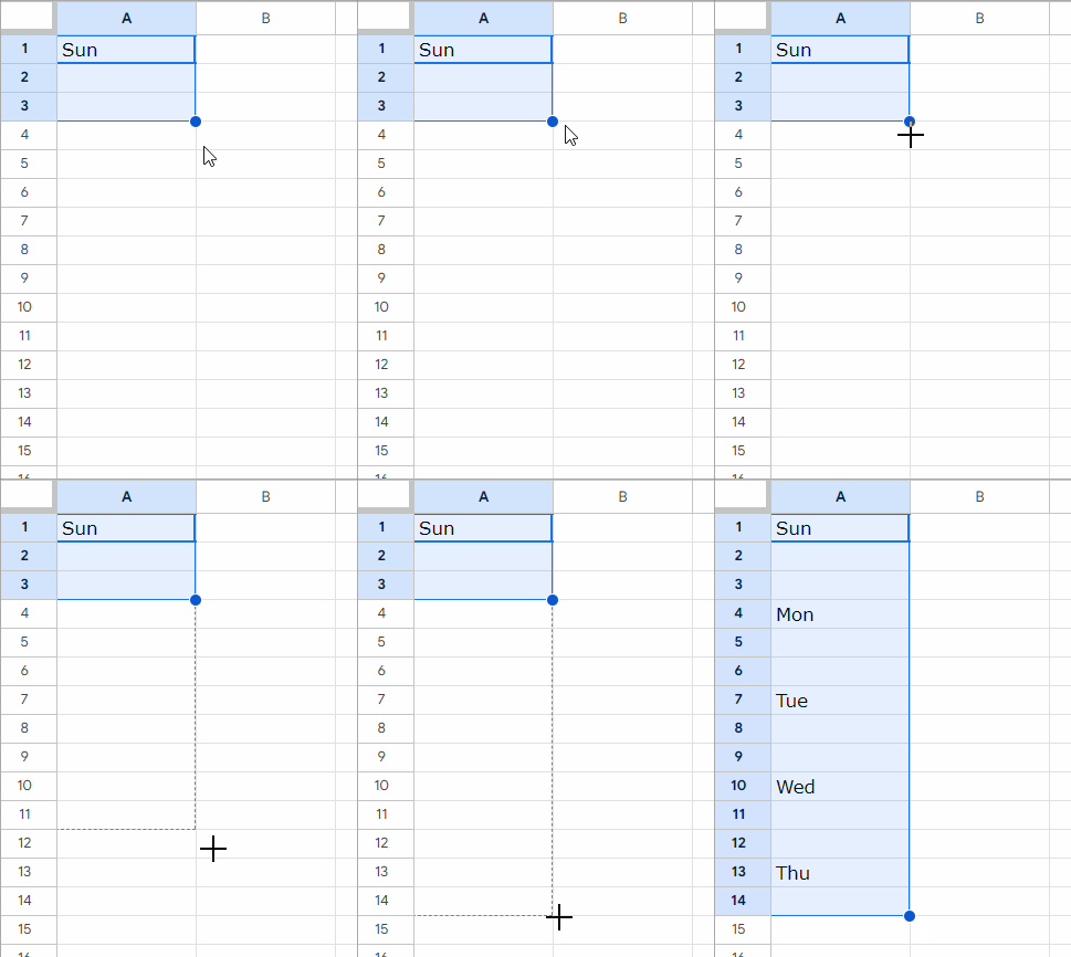
The above approach has two drawbacks:

Firstly, you can’t exclude weekends, or in other words, you can’t populate only the names of the weekdays.

Secondly, since it’s a manual approach, you won’t be able to use it in dynamic formulas when you want to populate days of the week as titles, for custom sorting, in lookups, etc.

Autofill Days of the Week Using an Array Formula

We can format sequence numbers 1 to 7 as days of the week. To achieve this, we need to use two functions in addition to ARRAYFORMULA: SEQUENCE and TEXT.

SEQUENCE is used for generating the sequence numbers, and TEXT is employed for formatting the numbers as days of the week. ARRAYFORMULA supports the TEXT function to expand results.

Before delving into the formula, let me clarify the logic.

In Google Sheets, actual dates are formatted numbers, where 1 corresponds to 31/12/1899. To test this, enter 1 in any cell and apply Format > Number > Date.

The day of the week for 31/12/1899 is Sunday. Consequently, the days of the week corresponding to the numbers 1 to 7 will be Sunday through Saturday.

Here is the array formula to autofill days of the week in Google Sheets:

=ArrayFormula(TEXT(SEQUENCE(7), "DDDD"))

To get abbreviated days (Sun to Sat), replace “DDDD” with “DDD”.

If you want to repeat the days of the week, replace 7 with 14 or the number of cells you want to fill. Here is an example:

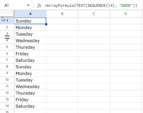
In the above examples, the first day of the week is Sunday. If you want the first day of the week to start from Monday, you need to modify the SEQUENCE. How?

In the above examples, we have followed the syntax SEQUENCE(rows), but use SEQUENCE(rows, columns, start) instead, where rows will be the number of rows to autofill, columns will be 1, and start will be 1 for Sunday, 2 for Monday, and so on.

Inserting Blank Rows Below Days of the Week:

This is a straightforward task. In a previous tutorial, I explained how to add blank rows below SEQUENCE results. We will apply that technique here.

Generic Formula:

=TOCOL(IFNA(HSTACK(autofill_formula,)))

In this formula, the comma (,) separator controls the number of blank rows inserted. For example, the following formula will autofill the days of the week with 3 blank rows in between:

=TOCOL(IFNA(HSTACK(ArrayFormula(TEXT(SEQUENCE(14), "DDDD")),,,)))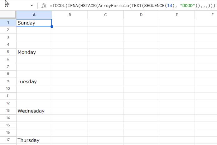

How to Autofill Weekday Names Using an Array Formula

As previously mentioned, we can treat the numbers as dates, allowing us to utilize the WORKDAY.INTL function to exclude specific weekends.

So, essentially, we will treat sequential numbers as dates and use the WORKDAY.INTL function to populate sequential dates excluding weekends. The text formatting will convert those dates (numbers, in other words) to weekday names.

Here is the formula to autofill weekday names in Google Sheets:

=ArrayFormula(TEXT(WORKDAY.INTL(1, SEQUENCE(20), "0000011"), "DDDD"))

This formula will autofill weekday names (Monday-Friday) in 20 cells.

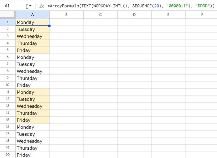
You can specify weekends of your choice by modifying the “0000011” part of the formula.

Specify weekends using seven 0s and 1s, where the first number represents Monday, and the last number is for Sunday. A zero indicates a workday, and a 1 indicates a weekend.

For example, “0000110” would mean Friday and Saturday are weekends.

Resources

With this tutorial, you can learn to autofill days of the week with or without weekends in a column. If you are familiar with SEQUENCE usage, you can also get the results in a row.

I mean, replace SEQUENCE(n) with SEQUENCE(1, n), where n is the number of values in the result. If that may confuse you, simply wrap the formulas with the TRANSPOSE or TOROW function.

Here are some additional resources to handle similar scenarios in Google Sheets:

1. Sort by Day of the Week in Google Sheets
2. How to Populate Sequential Dates Excluding Weekends in Google Sheets
3. Weekday Name to Weekday Number in Google Sheets
4. How to Get Sequence of Months in Google Sheets